Unlock document.
This document is partially blurred.
Unlock all pages and 1 million more documents.
Get Access
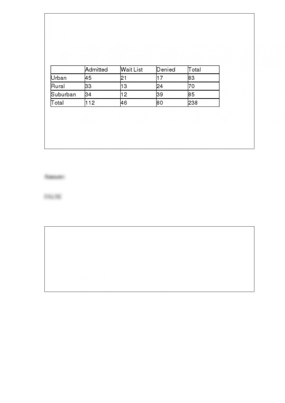
TABLE 12-11
The director of admissions at a state college is interested in seeing if admissions status
(admitted, waiting list, denied admission) at his college is independent of the type of
community in which an applicant resides. He takes a sample of recent admissions
decisions and forms the following table:
He will use this table to do a chi-square test of independence with a level of
significance of 0.01.
True or False: Referring to Table 12-11, the null hypothesis will be rejected.
True or False: TABLE 17-8
The superintendent of a school district wanted to predict the percentage of students
passing a sixth-grade proficiency test. She obtained the data on percentage of students
passing the proficiency test (% Passing), daily mean of the percentage of students
attending class (% Attendance), mean teacher salary in dollars (Salaries), and
instructional spending per pupil in dollars (Spending) of 47 schools in the state.
Following is the multiple regression output with Y = % Passing as the dependent
variable, X1 = % Attendance, X2 = Salaries and X3 = Spending:
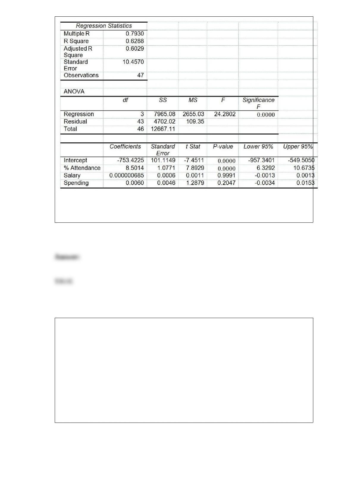
Referring to Table 17-8, the null hypothesis H0 : β1 = β2 = β3 = 0 implies that the
percentage of students passing the proficiency test is not related to any of the
explanatory variables.
TABLE 11-11
A student team in a business statistics course designed an experiment to investigate
whether the brand of bubblegum used affected the size of bubbles they could blow. To
reduce the person-to-person variability, the students decided to use a randomized block
design using themselves as blocks.
Four brands of bubblegum were tested. A student chewed two pieces of a brand of gum
and then blew a bubble, attempting to make it as big as possible. Another student
measured the diameter of the bubble at its biggest point. The following table gives the
diameters of the bubbles (in inches) for the 16 observations.
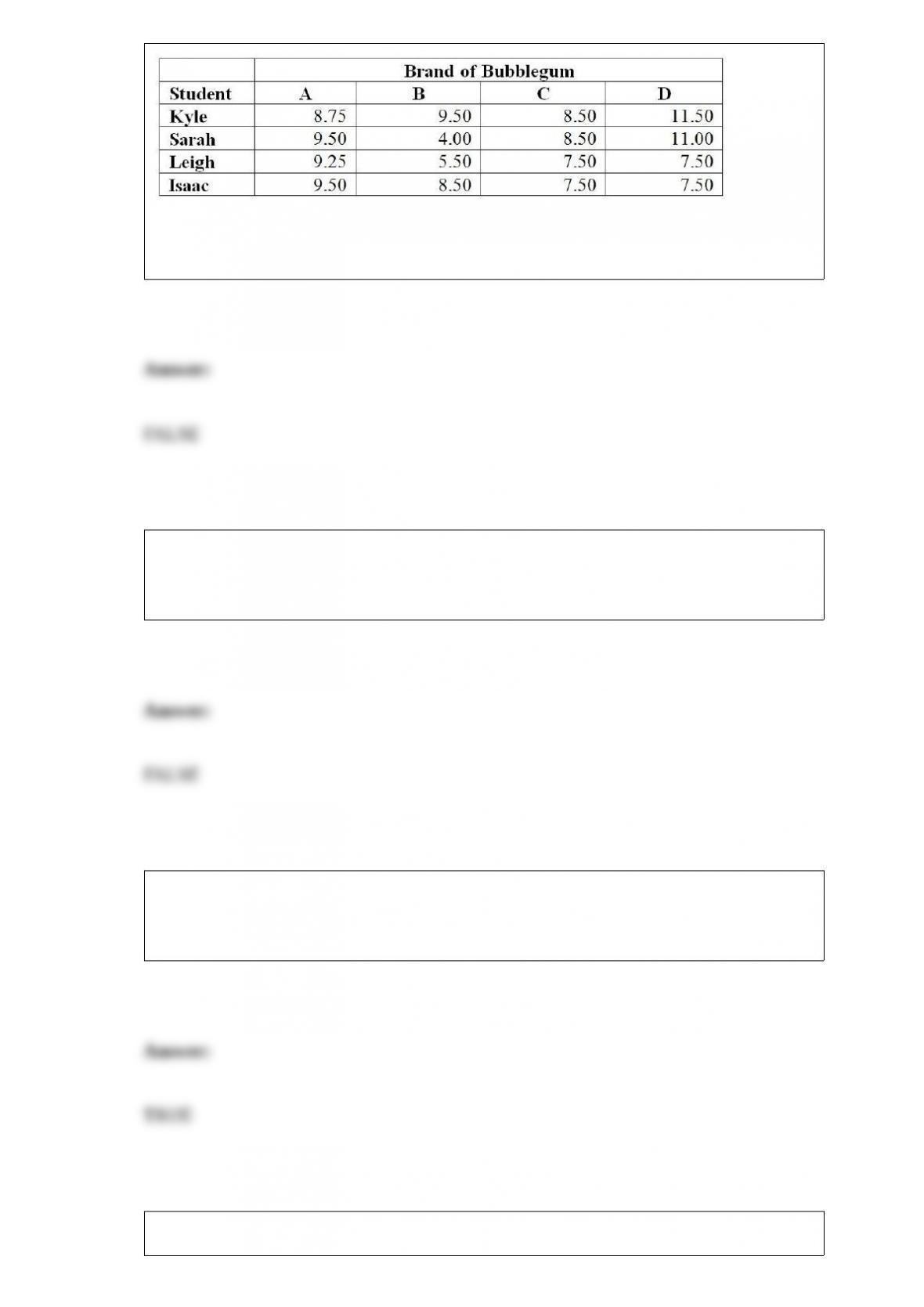
True or False: Referring to Table 11-11, the null hypothesis for the randomized block F
test for the difference in the means should be rejected at a 0.05 level of significance.
True or False: Referring to Table 14-16, the 0 to 60 miles per hour acceleration time of
a sedan is predicted to be 0.7264 seconds lower than that of a non-sedan with the same
engine size.
True or False: The confidence interval for the mean of Y is always narrower than the
prediction interval for an individual response Y given the same data set, X value, and
confidence level.
True or False: Some business analytics involve starting with many variables and are
then followed by filtering the data by exploring specific combinations of categorical
values or numerical range.
True or False: The diameters of 10 randomly selected bolts have a binomial
distribution.
True or False: A multidimensional contingency table allows you to tally the responses
of more than two continuous variables.
True or False: In selecting a forecasting model, you should perform a residual analysis.
True or False: If the amount of gasoline purchased per car at a large service station has
a population mean of 15 gallons and a population standard deviation of 4 gallons, and a
random sample of 4 cars is selected, there is approximately a 68.26% chance that the
sample mean will be between 13 and 17 gallons.
True or False: A Marine drill instructor recorded the time in which each of 11 recruits
completed an obstacle course both before and after basic training. To test whether any
improvement occurred, the instructor would use a t-distribution with 11 degrees of
freedom.
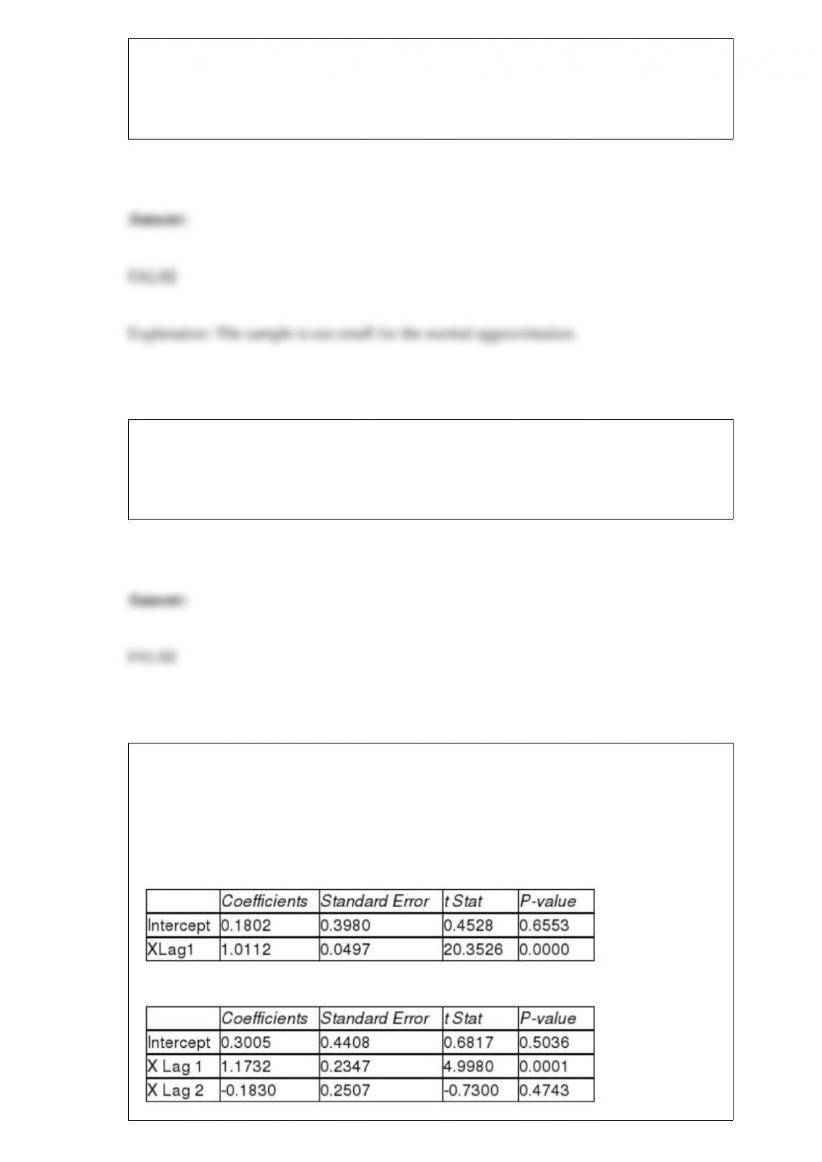
TABLE 16-9
Given below are EXCEL outputs for various estimated autoregressive models for a
company's real operating revenues (in billions of dollars) from 1989 to 2012. From the
data, you also know that the real operating revenues for 2010, 2011, and 2012 are
11.7909, 11.7757 and 11.5537, respectively.
First-Order Autoregressive Model:
Second-Order Autoregressive Model:
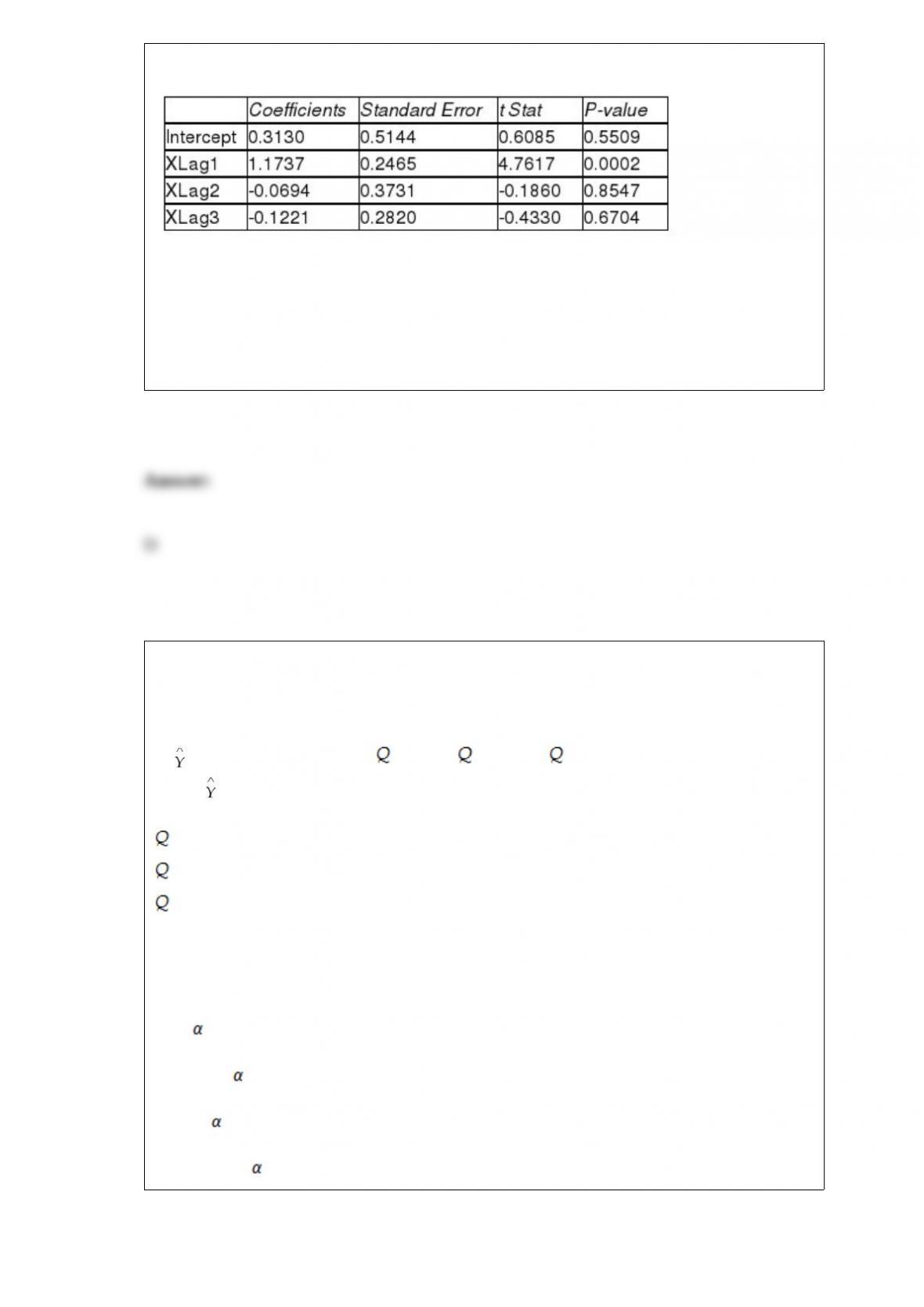
Third-Order Autoregressive Model:
Referring to Table 16-9, if one decides to use the Third-Order Autoregressive model,
what will the predicted real operating revenue for the company be in 2014?
A) $11.55 billion
B) $11.62 billion
C) $12.47 billion
D) $12.57 billion
TABLE 16-14
A contractor developed a multiplicative time-series model to forecast the number of
contracts in future quarters, using quarterly data on number of contracts during the
3-year period from 2010 to 2012. The following is the resulting regression equation:
ln = 3.37 + 0.117 X - 0.083 1 + 1.28 2 + 0.617 3
where is the estimated number of contracts in a quarter
X is the coded quarterly value with X = 0 in the first quarter of 2010
1 is a dummy variable equal to 1 in the first quarter of a year and 0 otherwise
2 is a dummy variable equal to 1 in the second quarter of a year and 0 otherwise
3 is a dummy variable equal to 1 in the third quarter of a year and 0 otherwise
Referring to Table 16-14, in testing the coefficient of X in the regression equation
(0.117) the results were a t-statistic of 9.08 and an associated p-value of 0.0000. Which
of the following is the best interpretation of this result?
A) The quarterly growth rate in the number of contracts is significantly different from
0% ( = 0.05).
B) The quarterly growth rate in the number of contracts is not significantly different
from 0% ( = 0.05).
C) The quarterly growth rate in the number of contracts is significantly different from
100% ( = 0.05).
D) The quarterly growth rate in the number of contracts is not significantly different
from 100% ( = 0.05).

TABLE 1-3
The manager of the customer service division of a major consumer electronics company
is interested in determining whether the customers who have purchased a Blu-ray
player made by the company over the past 12 months are satisfied with their products.
Referring to Table 1-3, if a customer survey questionnaire is included in all the Blu-ray
players made and sold by the company over the past 12 months, this method of
collecting data will most like suffer from
A) nonresponse error.
B) measurement error.
C) coverage error.
D) nonprobability sampling.
TABLE 16-7
The executive vice-president of a drug manufacturing firm believes that the demand for
the firm's most popular drug has been evidencing an exponential trend since 1999. She
uses Microsoft Excel to obtain the partial output below. The dependent variable is the
log base 10 of the demand for the drug, while the independent variable is years, where
1999 is coded as 0, 2000 is coded as 1, etc.
SUMMARY OUTPUT
Referring to Table 16-7, the forecast for the demand in 2016 is ________.
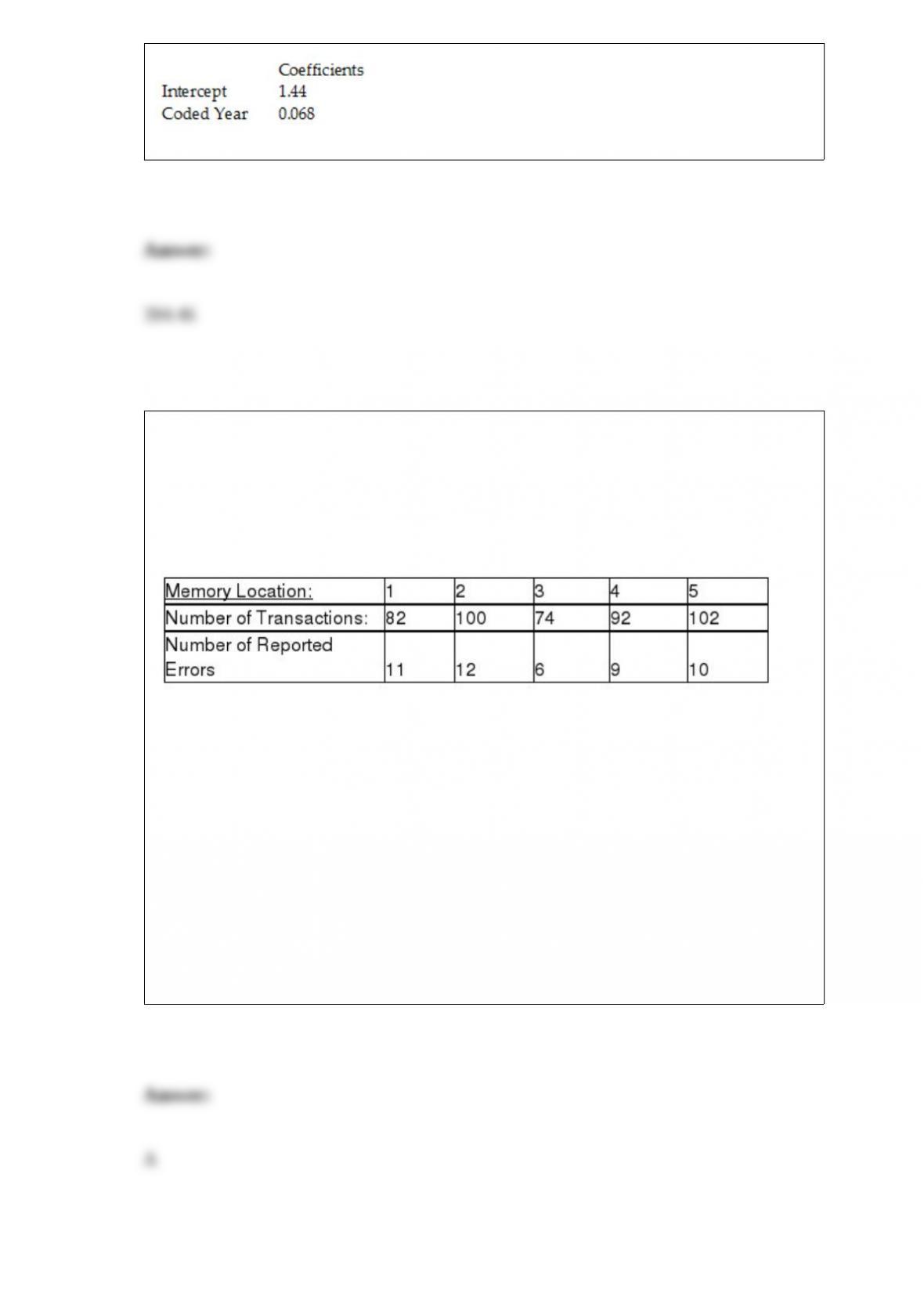
TABLE 12-4
A computer used by a 24-hour banking service is supposed to randomly assign each
transaction to one of 5 memory locations. A check at the end of a day's transactions
gave the counts shown in the table to each of the 5 memory locations, along with the
number of reported errors.
The bank manager wanted to test whether the proportion of errors in transactions
assigned to each of the 5 memory locations differ.
Referring to Table 12-4, the degrees of freedom of the test statistic is
A) 4.
B) 8.
C) 10.
D) 448.

Referring to Table 14-17, which of the following is a correct
statement?
TABLE 14-17
Given below are results from the regression analysis where the
dependent variable is the number of weeks a worker is unemployed
due to a layo% (Unemploy) and the independent variables are the age
of the worker (Age) and a dummy variable for management position
(Manager: 1 = yes, 0 = no).
The results of the regression analysis are given below:
A) 37.65% of the total variation in the number of weeks a worker is
unemployed due to a layo% can be explained by the age of the worker
and whether the worker is a manager.
B) 37.65% of the total variation in the number of weeks a worker is
unemployed due to a layo% can be explained by the age of the worker
and whether the worker is a manager after adjusting for the number
of predictors and sample size.
C) 37.65% of the total variation in the number of weeks a worker is
unemployed due to a layo% can be explained by the age of the worker
and whether the worker is a manager after adjusting for the level of
signiticance.
D) 37.65% of the total variation in the number of weeks a worker is
unemployed due to a layo% can be explained by the age of the worker
and whether the worker is a manager holding constant the effect of
all the independent variables.
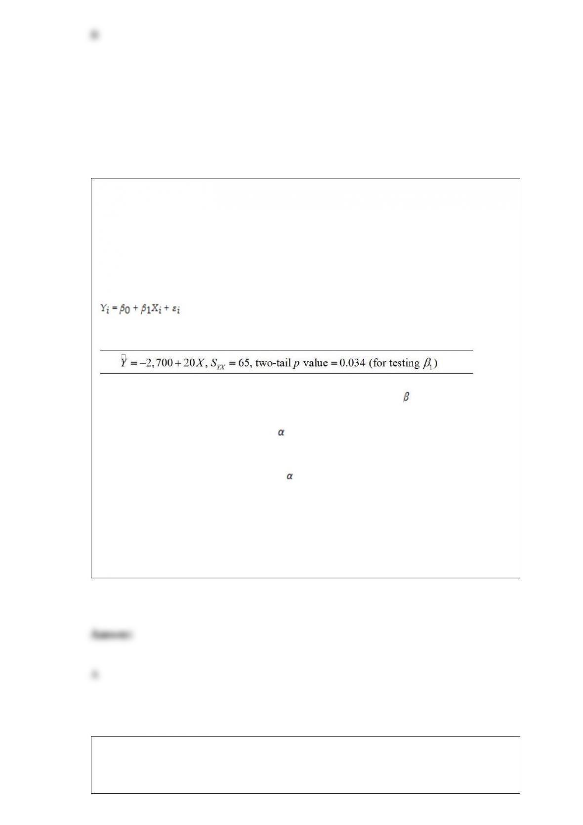
TABLE 13-1
A large national bank charges local companies for using their services. A bank official
reported the results of a regression analysis designed to predict the bank's charges (Y) -
measured in dollars per month - for services rendered to local companies. One
independent variable used to predict service charges to a company is the company's
sales revenue (X) - measured in millions of dollars. Data for 21 companies who use the
bank's services were used to fit the model:
The results of the simple linear regression are provided below.
Referring to Table 13-1, interpret the p-value for testing whether 1exceeds 0.
A) There is sufficient evidence (at the = 0.05) to conclude that sales revenue (X) is a
useful linear predictor of service charge (Y).
B) There is insufficient evidence (at the = 0.10) to conclude that sales revenue (X) is a
useful linear predictor of service charge (Y).
C) Sales revenue (X) is a poor predictor of service charge (Y).
D) For every $1 million increase in sales revenue, you expect a service charge to
increase $0.034.
Referring to Table 14-19, which of the following is the correct
interpretation for the Income slope coe9cient?

TABLE 14-19
The marketing manager for a nationally franchised lawn service
company would like to study the characteristics that differentiate
home owners who do and do not have a lawn service. A random
sample of 30 home owners located in a suburban area near a large
city was selected; 11 did not have a lawn service (code 0) and 19 had
a lawn service (code 1). Additional information available concerning
these 30 home owners includes family income (Income, in thousands
of dollars) and lawn size (Lawn Size, in thousands of square feet).
The PHStat output is given below:
A) Holding constant the effect of lawn size, the estimated number of
lawn services purchased increases by 0.0304 for each increase of one
thousand dollars in family income.
B) Holding constant the effect of lawn size, the estimated average
number of lawn services purchased increases by 0.0304 for each
increase of one thousand dollars in family income.
C) Holding constant the effect of lawn size, the estimated probability
of purchasing a lawn service increases by 0.0304 for each increase of
one thousand dollars in family income.
D) Holding constant the effect of lawn size, the estimated natural
logarithm of the odds ratio of purchasing a lawn service increases by
0.0304 for each increase of one thousand dollars in family income.
TABLE 17-6
A weight-loss clinic wants to use regression analysis to build a model for weight loss of
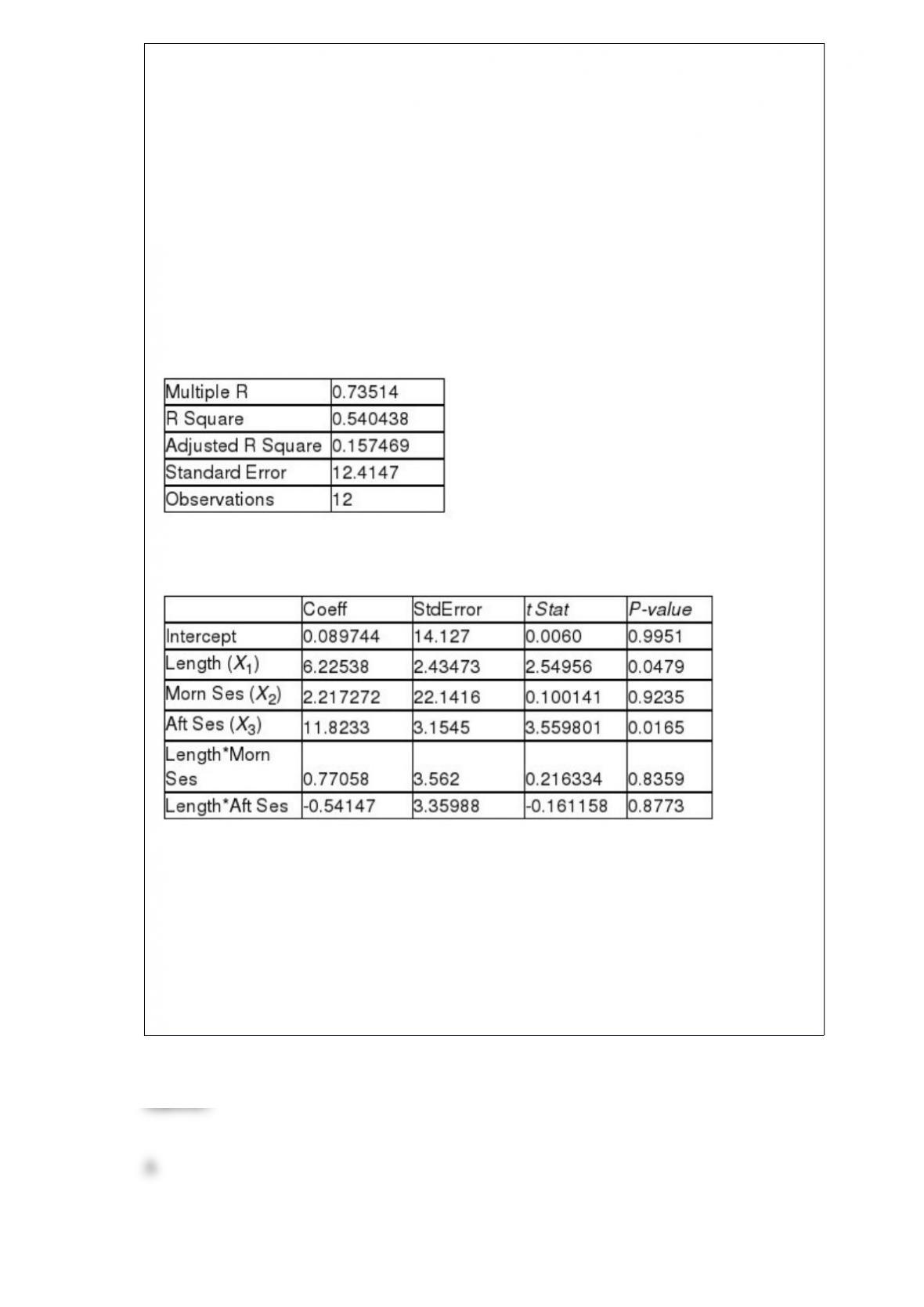
a client (measured in pounds). Two variables thought to affect weight loss are client's
length of time on the weight-loss program and time of session. These variables are
described below:
Y = Weight loss (in pounds)
X1 = Length of time in weight-loss program (in months)
X2 = 1 if morning session, 0 if not
X3 = 1 if afternoon session, 0 if not (Base level = evening session)
Data for 12 clients on a weight-loss program at the clinic were collected and used to fit
the interaction model:
Y = β0 + β1X1 + β2X2 + β3X3 + β4X1X2 + β5X1X3 + ε
Partial output from Microsoft Excel follows:
Regression Statistics
ANOVA
F = 5.41118 Significance F = 0.040201
Referring to Table 17-6, in terms of the βs in the model, give the mean change in
weight loss (Y) for every 1-month increase in time in the program (X1) when attending
the morning session.
A) β1 + β4
B) β1 + β5
C) β1
D) β4 + β5

The probability that house sales will increase in the next 6 months is estimated to be
0.25. The probability that the interest rates on housing loans will go up in the same
period is estimated to be 0.74. The probability that house sales or interest rates will go
up during the next 6 months is estimated to be 0.89. The probability that neither house
sales nor interest rates will increase during the next 6 months is
A) 0.11.
B) 0.195.
C) 0.89.
D) 0.90.
In a binomial distribution,
A) the variable X is continuous.
B) the probability of event of interest is stable from trial to trial.
C) the number of trials n must be at least 30.
D) the results of one trial are dependent on the results of the other trials.
A major Blu-ray rental chain is considering opening a new store in an area that
currently does not have any such stores. The chain will open if there is evidence that
more than 5,000 of the 20,000 households in the area are equipped with Blu-ray
players. It conducts a telephone poll of 300 randomly selected households in the area
and finds that 96 have Blu-ray players. The value of the test statistic in this problem is
approximately equal to

A) 2.80.
B) 2.60.
C) 1.94.
D) 1.30.
A manager of the credit department for an oil company would like to determine whether
the mean monthly balance of credit card holders is equal to $75. An auditor selects a
random sample of 100 accounts and finds that the mean owed is $83.40 with a sample
standard deviation of $23.65. If you wanted to test whether the mean balance is
different from $75 and decided to reject the null hypothesis, what conclusion could you
reach?
A) There is no evidence that the mean balance is $75.
B) There is no evidence that the mean balance is not $75.
C) There is evidence that the mean balance is $75.
D) There is evidence that the mean balance is not $75.
TABLE 2-14
The table below contains the number of people who own a portable Blu-ray player in a
sample of 600 broken down by gender.
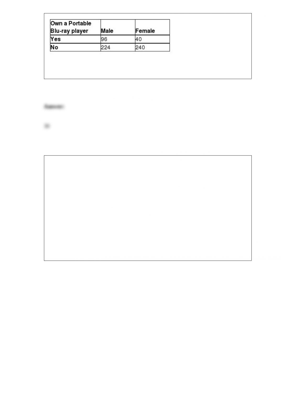
Referring to Table 2-14, of the males in the sample, ________ percent owned a portable
Blu-ray player.
TABLE 17-9
What are the factors that determine the acceleration time (in sec.) from 0 to 60 miles per
hour of a car? Data on the following variables for 171 different vehicle models were
collected:
Accel Time: Acceleration time in sec.
Cargo Vol: Cargo volume in cu. ft.
HP: Horsepower
MPG: Miles per gallon
SUV: 1 if the vehicle model is an SUV with Coupe as the base when SUV and Sedan
are both 0
Sedan: 1 if the vehicle model is a sedan with Coupe as the base when SUV and Sedan
are both 0
The regression results using acceleration time as the dependent variable and the
remaining variables as the independent variables are presented below.
The various residual plots are as shown below.
The coefficient of partial determination ( ) of each of the 5
predictors are, respectively, 0.0380, 0.4376, 0.0248, 0.0188, and 0.0312.
The coefficient of multiple determination for the regression model using each of the 5

variables Xj as the dependent variable and all other X variables as independent variables
( ) are, respectively, 0.7461, 0.5676, 0.6764, 0.8582, 0.6632.
Referring to Table 17-9, what is the p-value of the test statistic to determine whether
MPG makes a significant contribution to the regression model in the presence of the
other independent variables at a 5% level of significance?
TABLE 6-6
According to Investment Digest, the arithmetic mean of the annual return for common
stocks over an 85-year period was 9.5%, but the value of the variance was not
mentioned. Also 25% of the annual returns were below 8%, while 65% of the annual
returns were between 8% and 11.5%. The article claimed that the distribution of annual
return for common stocks was bell-shaped and approximately symmetric. Assume that
this distribution is normal with the mean given above. Answer the following questions
without the help of a calculator, statistical software or statistical table.
Referring to Table 6-6, find the probability that the annual return of a random year will
be less than 7.5%.
Referring to Table 14-10, the regression sum of squares that is
missing in the ANOVA table should be ________.
TABLE 14-10
You worked as an intern at We Always Win Car Insurance Company
last summer. You notice that individual car insurance premiums
depend very much on the age of the individual and the number of
traffic tickets received by the individual. You performed a regression

analysis in EXCEL and obtained the following partial information:
Referring to Table 14-18, what is the estimated odds ratio for a school
with a mean SAT score of 1100 and a TOEFL criterion that is not at
least 90?
TABLE 14-18
A logistic regression model was estimated in order to predict the
probability that a randomly chosen university or college would be a
private university using information on mean total Scholastic Aptitude
Test score (SAT) at the university or college and whether the TOEFL
criterion is at least 90 (Toe90 = 1 if yes, 0 otherwise). The
dependent variable, Y, is school type (Type = 1 if private and 0
otherwise).
The PHStat output is given below:

TABLE 8-1
The managers of a company are worried about the morale of their employees. In order
to determine if a problem in this area exists, they decide to evaluate the attitudes of their
employees with a standardized test. They select the Fortunato test of job satisfaction,
which has a known standard deviation of 24 points.
Referring to Table 8-1, they should sample ________ employees if they want to
estimate the mean score of the employees within 5 points with 90% confidence.


