TABLE 15-6
Given below are results from the regression analysis on 40 observations where the
dependent variable is the number of weeks a worker is unemployed due to a layoff (Y)
and the independent variables are the age of the worker (X1), the number of years of
education received (X2), the number of years at the previous job (X3), a dummy variable
for marital status (X4: 1 = married, 0 = otherwise), a dummy variable for head of
household (X5: 1 = yes, 0 = no) and a dummy variable for management position (X6: 1
= yes, 0 = no).
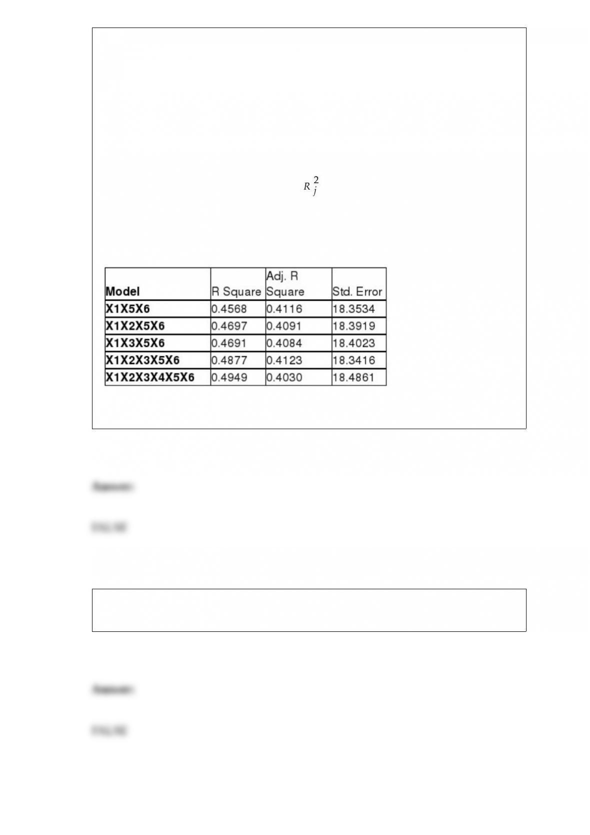
The coefficient of multiple determination ( ) for the regression model using each of
the 6 variables Xj as the dependent variable and all other X variables as independent
variables are, respectively, 0.2628, 0.1240, 0.2404, 0.3510, 0.3342 and 0.0993.
The partial results from best-subset regression are given below:
True or False: Referring to Table 15-6, there is reason to suspect collinearity between
some pairs of predictors based on the values of the variance inflationary factor.
True or False: If the sample sizes in each group is larger than 5, the Kruskal-Wallis rank
test statistic can be approximated by a standardized normal distribution.

TABLE 12-11
The director of admissions at a state college is interested in seeing if admissions status
(admitted, waiting list, denied admission) at his college is independent of the type of
community in which an applicant resides. He takes a sample of recent admissions
decisions and forms the following table:
He will use this table to do a chi-square test of independence with a level of
significance of 0.01.
True or False: Referring to Table 12-11, the same decision would be made with this test
if the level of significance had been 0.05.
True or False: TABLE 17-10
Given below are results from the regression analysis where the dependent variable is
the number of weeks a worker is unemployed due to a layoff (Unemploy) and the
independent variables are the age of the worker (Age), the number of years of education
received (Edu), the number of years at the previous job (Job Yr), a dummy variable for
marital status (Married: 1 = married, 0 = otherwise), a dummy variable for head of
household (Head: 1 = yes, 0 = no) and a dummy variable for management position
(Manager: 1 = yes, 0 = no). We shall call this Model 1. The coefficient of partial
determination ( ) of each of the 6 predictors are, respectively,
0.2807, 0.0386, 0.0317, 0.0141, 0.0958, and 0.1201.
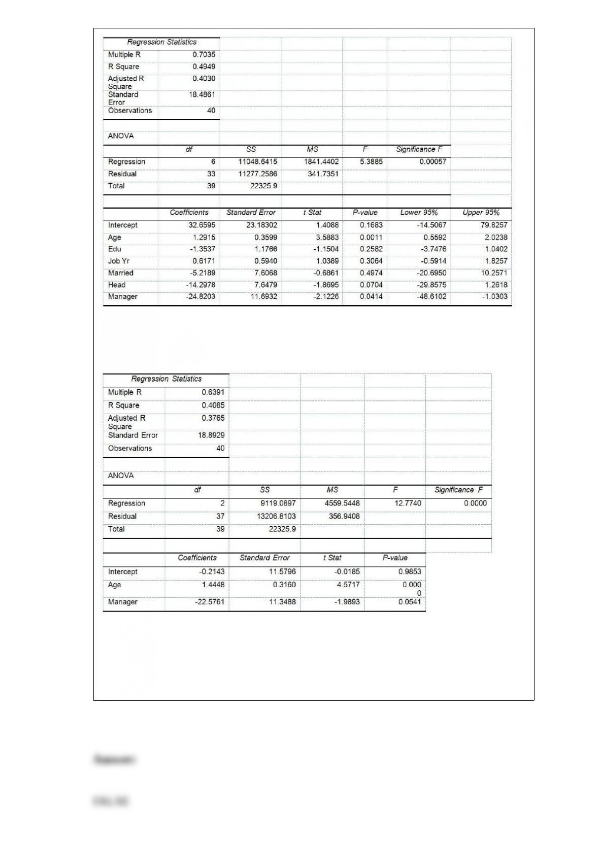
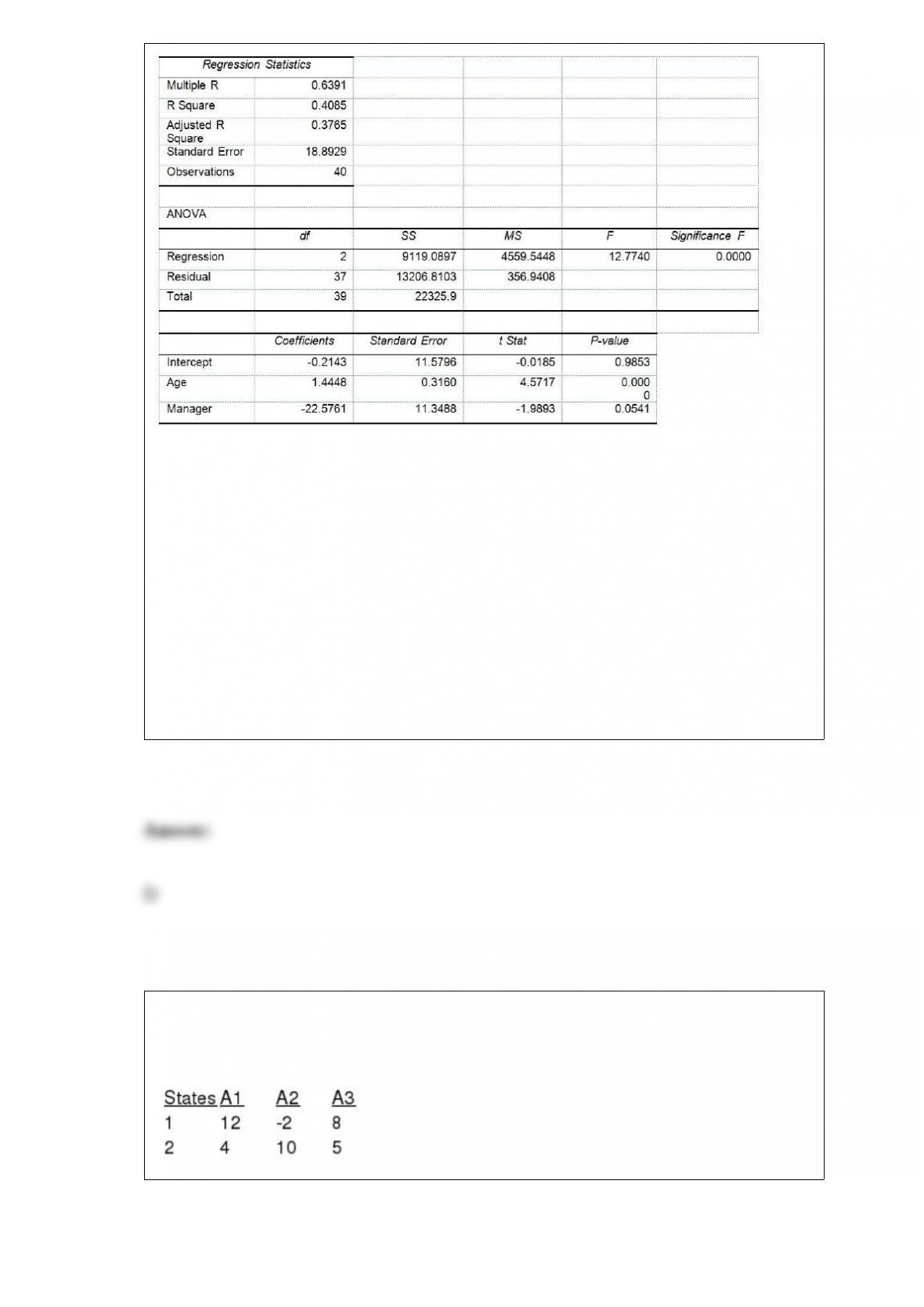
Model 2 is the regression analysis where the dependent variable is Unemploy and the
independent variables are Age and Manager. The results of the regression analysis are
given below:
Referring to Table 17-10, Model 1, we can conclude that, holding constant the effect of
the other independent variables, there is a difference in the mean number of weeks a
worker is unemployed due to a layoff between a worker who is married and one who is
not at a 5% level of significance if we use only the information of the 95% confidence
interval estimate for β4.
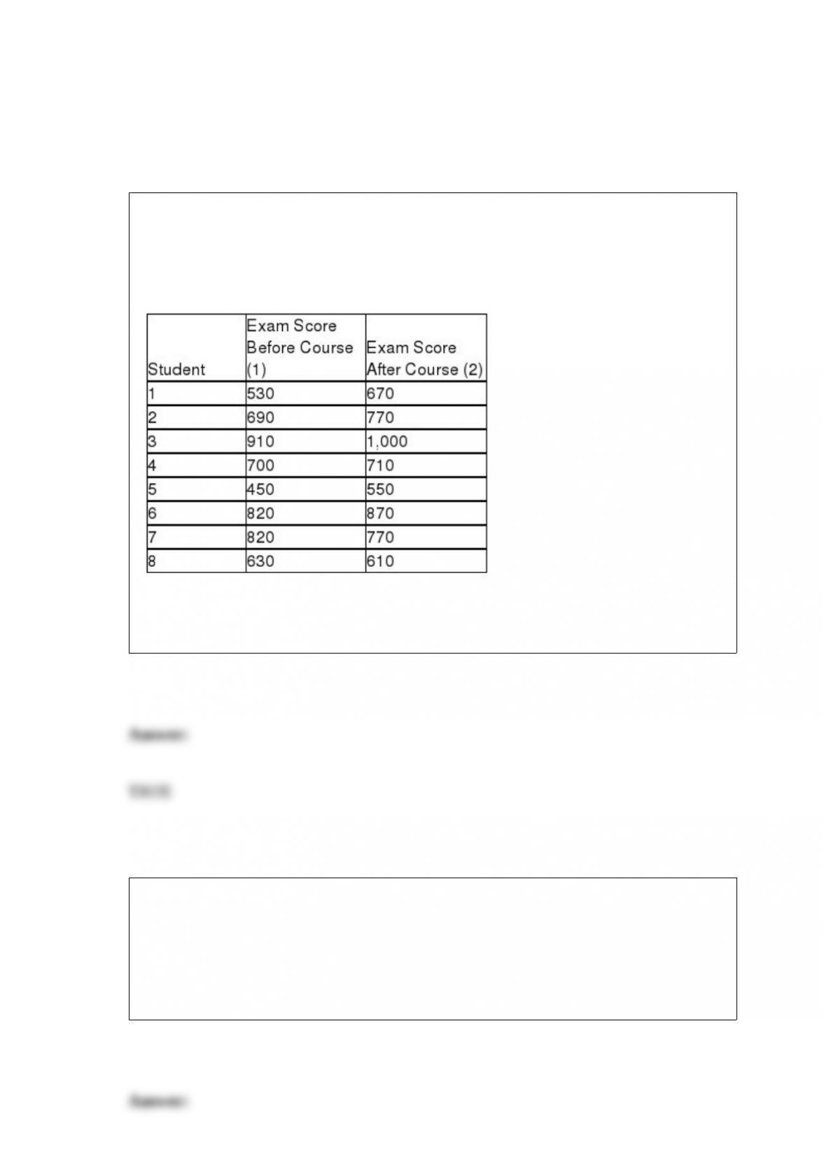
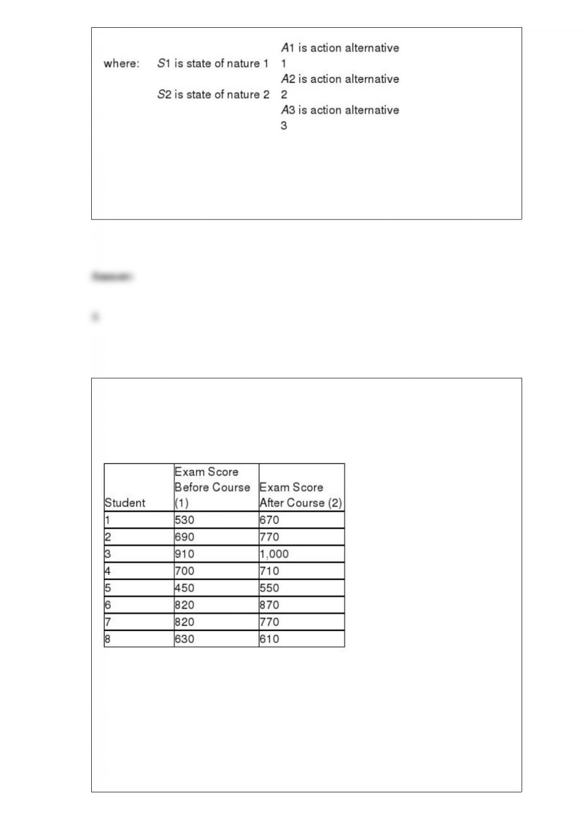
TABLE 10-5
To test the effectiveness of a business school preparation course, 8 students took a
general business test before and after the course. The results are given below.
True or False: Referring to Table 10-5, you must assume that the population of
difference scores is normally distributed.
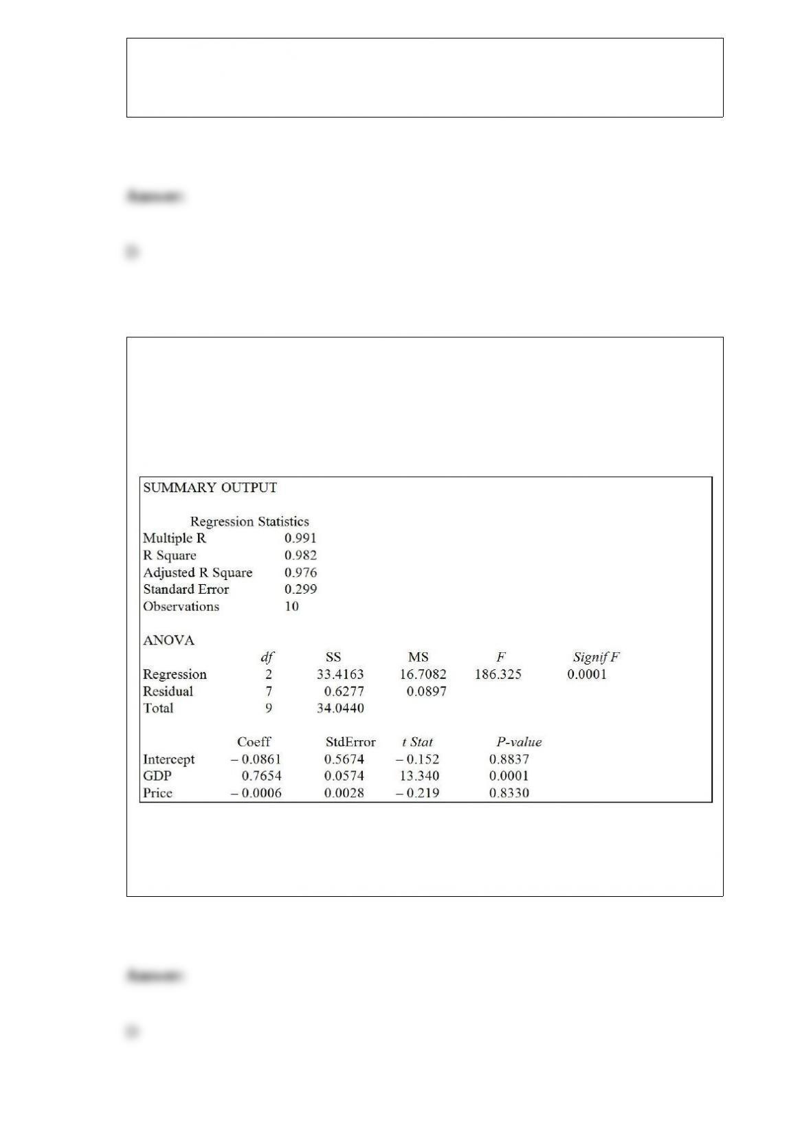
Referring to Table 14-3, to test for the significance of the coefficient on aggregate price
index, the p-value is
A) 0.0001.
B) 0.8330.
C) 0.8837.
D) 0.9999.
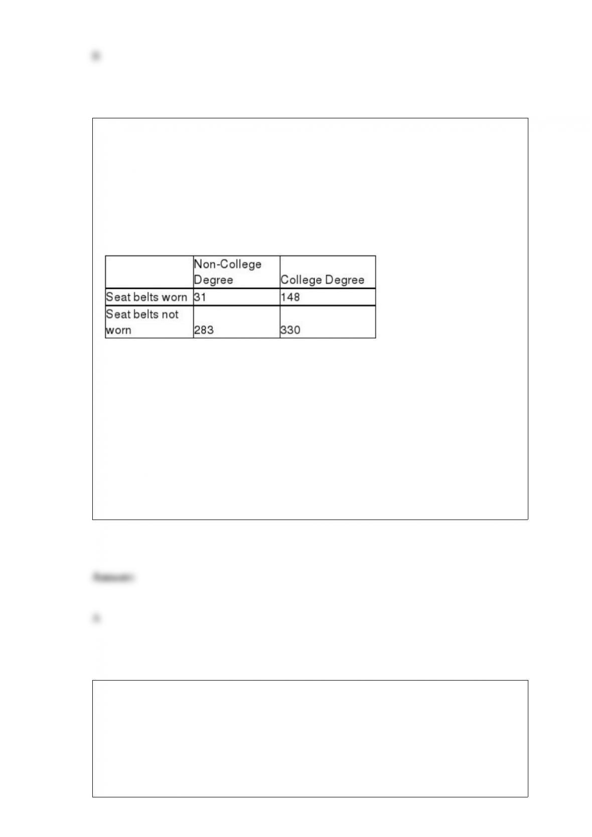
TABLE 12-8
A study was conducted to determine whether the use of seat belts in motor vehicles
depends on the educational status of the parents. A sample of 792 children treated for
injuries sustained from motor vehicle accidents was obtained, and each child was
classified according to (1) parents’ educational status (College Degree or Non-College
Degree) and (2) seat belt usage (worn or not worn) during the accident. The number of
children in each category is given in the table below.
Referring to Table 12-8, which test would be used to properly analyze the data in this
experiment?
A) X2 test for independence
B) X2 test for differences among more than two proportions
C) Wilcoxon rank sum test for independent populations
D) Kruskal-Wallis rank test
For a sample size of 1, the sampling distribution of the mean will be normally
distributed
A) regardless of the shape of the population.
B) only if the shape of the population is symmetrical.
C) only if the population values are positive.
D) only if the population is normally distributed.
Referring to Table 14-3, the p-value for GDP is
TABLE 14-3
An economist is interested to see how consumption for an economy (in $ billions) is
influenced by gross domestic product ($ billions) and aggregate price (consumer price
index). The Microsoft Excel output of this regression is partially reproduced below.
A) 0.05.
B) 0.01.
C) 0.001.
D) None of the above.
Which of the following is an assumption required by the Analysis of Proportions
(ANOP)?
A) The variance of the groups is different.
B) The observations from each of the groups are assumed to be approximately normally
distributed.
C) The shape of the distribution of the observations from the groups is different.
D) The number of observations in each group has to be large.
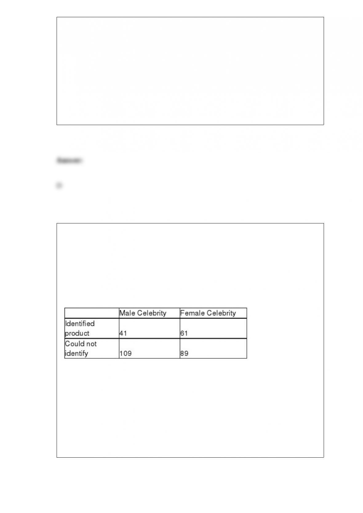
TABLE 12-9
Many companies use well-known celebrities as spokespersons in their TV
advertisements. A study was conducted to determine whether brand awareness of
female TV viewers and the gender of the spokesperson are independent. Each in a
sample of 300 female TV viewers was asked to identify a product advertised by a
celebrity spokesperson. The gender of the spokesperson and whether or not the viewer
could identify the product was recorded. The numbers in each category are given below.
Referring to Table 12-9, the degrees of freedom of the test statistic are
A) 1.
B) 2.
C) 4.
D) 299.
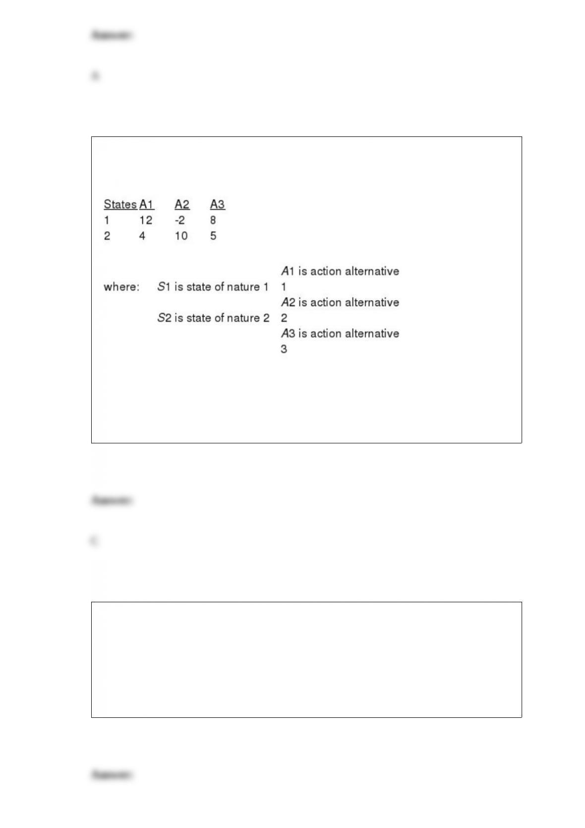
TABLE 19-1
The following payoff table shows profits associated with a set of 3 alternatives under 2
possible states of nature
Referring to Table 19-1, the opportunity loss for A3 when S2 occurs is
A) 0.
B) 4.
C) 5.
D) 6.
An investor wanted to forecast the price of a certain stock. He collected the mean daily
price for the stock over the past 10 years. Which of the following would be the most
appropriate analysis to perform?
A) The Marascuilo Procedure
B) The Tukey-Kramer Procedure
C) Least-squares forecasting with monthly or quarterly data
D) Autoregressive modeling

How many tissues should the Kimberly Clark Corporation package of Kleenex contain?
Researchers determined that 60 tissues is the mean number of tissues used during a
cold. Suppose a random sample of 100 Kleenex users yielded the following data on the
number of tissues used during a cold: = 52,
S = 22. Suppose the test statistic does fall in the rejection region at = 0.05. Which of
the following decisions is correct?
A) At = 0.05, you do not reject H0.
B) At = 0.05, you reject H0.
C) At = 0.10, you do not reject H0.
D) At = 0.10, you reject H0.
TABLE 17-10
Given below are results from the regression analysis where the dependent variable is
the number of weeks a worker is unemployed due to a layoff (Unemploy) and the
independent variables are the age of the worker (Age), the number of years of education
received (Edu), the number of years at the previous job (Job Yr), a dummy variable for
marital status (Married: 1 = married, 0 = otherwise), a dummy variable for head of
household (Head: 1 = yes, 0 = no) and a dummy variable for management position
(Manager: 1 = yes, 0 = no). We shall call this Model 1. The coefficient of partial
determination ( ) of each of the 6 predictors are, respectively,
0.2807, 0.0386, 0.0317, 0.0141, 0.0958, and 0.1201.
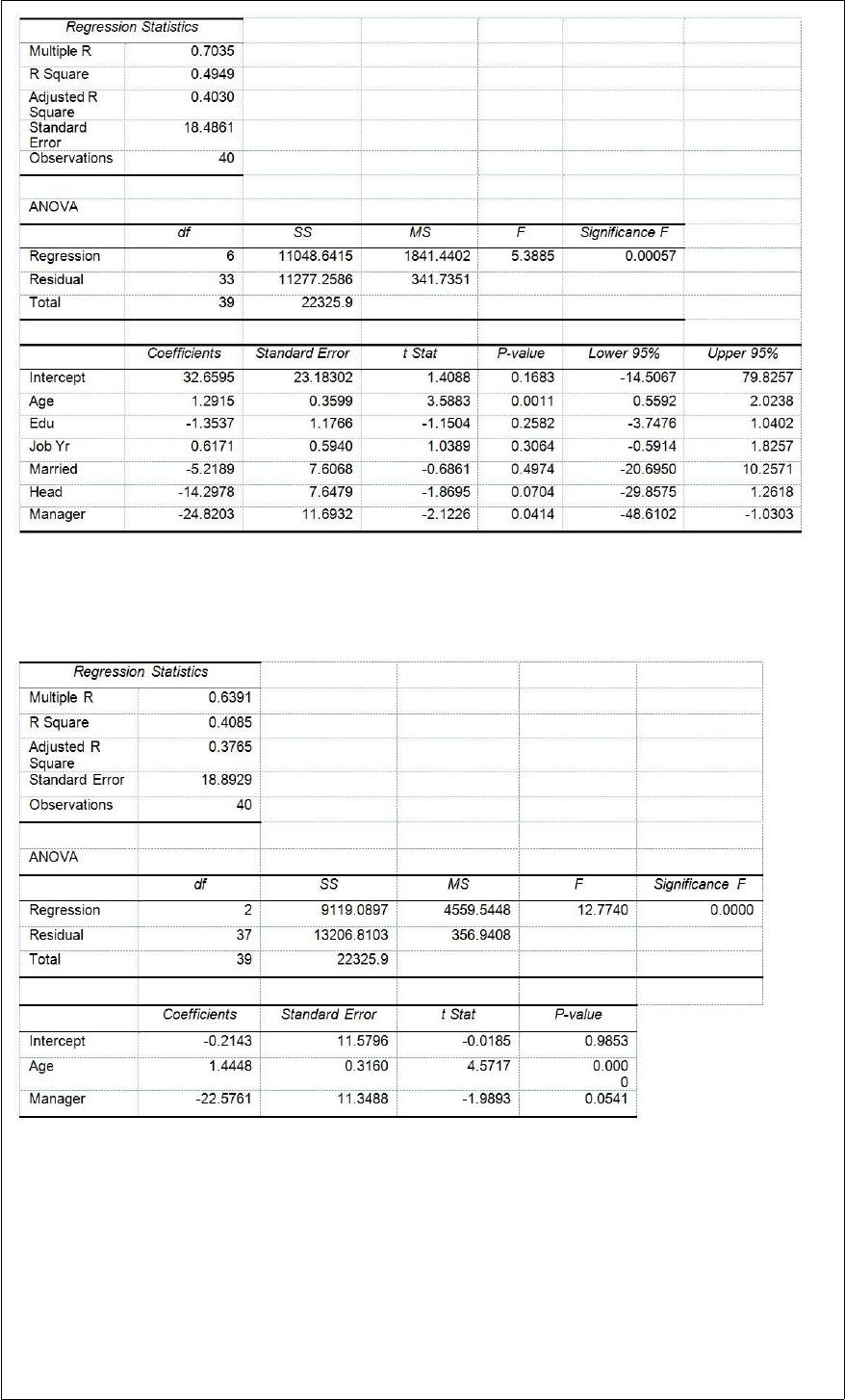
Model 2 is the regression analysis where the dependent variable is Unemploy and the
independent variables are Age and Manager. The results of the regression analysis are
given below:
Referring to Table 17-10, Model 1, which of the following is the correct alternative
hypothesis to test whether age has any effect on the number of weeks a worker is
unemployed due to a layoff while holding constant the effect of all the other
independent variables?
A) H1 : β0 ≠0
B) H1 : β1 ≠0
C) H1 : β2 ≠0
D) H1 : β3 ≠0
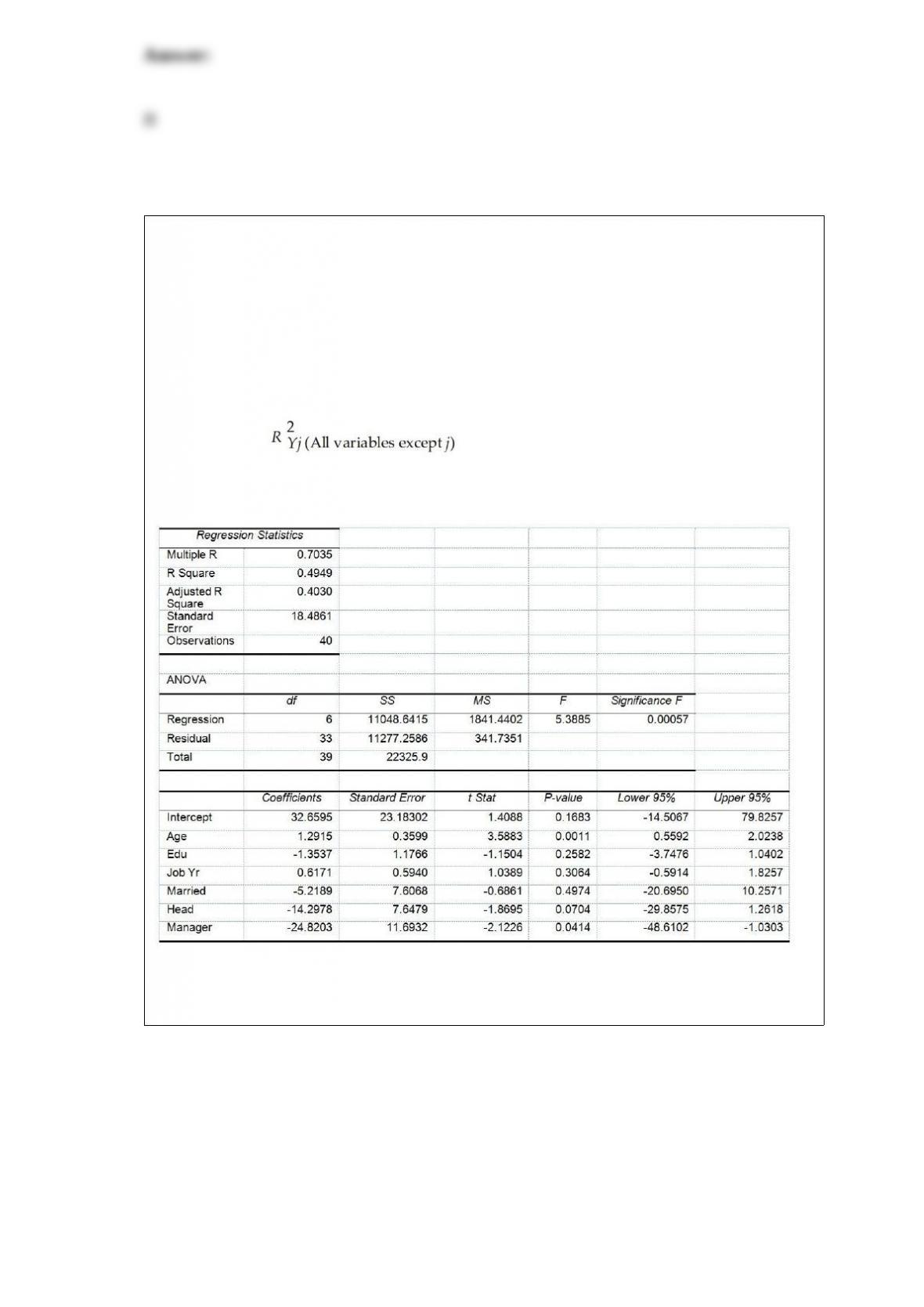
TABLE 17-10
Given below are results from the regression analysis where the dependent variable is
the number of weeks a worker is unemployed due to a layoff (Unemploy) and the
independent variables are the age of the worker (Age), the number of years of education
received (Edu), the number of years at the previous job (Job Yr), a dummy variable for
marital status (Married: 1 = married, 0 = otherwise), a dummy variable for head of
household (Head: 1 = yes, 0 = no) and a dummy variable for management position
(Manager: 1 = yes, 0 = no). We shall call this Model 1. The coefficient of partial
determination ( ) of each of the 6 predictors are, respectively,
0.2807, 0.0386, 0.0317, 0.0141, 0.0958, and 0.1201.
Model 2 is the regression analysis where the dependent variable is Unemploy and the
independent variables are Age and Manager. The results of the regression analysis are
given below:
Referring to Table 17-10, Model 1, which of the following is a correct statement?
A) On average, those who are in a management position are estimated to stay jobless
shorter by approximately 1.35 weeks while holding constant the effects of all the
remaining independent variables.
B) On average, those who are in a management position are estimated to stay jobless
shorter by approximately 5.22 weeks while holding constant the effects of all the
remaining independent variables.
C) On average, those who are in a management position are estimated to stay jobless
shorter by approximately 14.30 weeks while holding constant the effects of all the
remaining independent variables.
D) On average, those who are in a management position are estimated to stay jobless
shorter by approximately 24.82 weeks while holding constant the effects of all the
remaining independent variables.
TABLE 19-1
The following payoff table shows profits associated with a set of 3 alternatives under 2
possible states of nature
Referring to Table 19-1, what is the best action using the maximax criterion?
A) Action A1
B) Action A2
C) Action A3
D) It cannot be determined.
TABLE 10-5
To test the effectiveness of a business school preparation course, 8 students took a
general business test before and after the course. The results are given below.
Referring to Table 10-5, the value of the sample mean difference is ________ if the
difference scores reflect the results of the exam after the course minus the results of the
exam before the course.
A) 0
B) 50

C) 68
D) 400
You use the finite population correction factor when
A) you sample without replacement and the sample size is larger than 5% of the
population size.
B) you sample without replacement and the sample size is smaller than 5% of the
population size.
C) you sample with replacement and the sample size is larger than 5% of the population
size.
D) you sample with replacement and the sample size is smaller than 5% of the
population size.
TABLE 11-2
A realtor wants to compare the mean sales-to-appraisal ratios of residential properties
sold in four neighborhoods (A, B, C, and D). Four properties are randomly selected
from each neighborhood and the ratios recorded for each, as shown below.
Interpret the results of the analysis summarized in the following table:
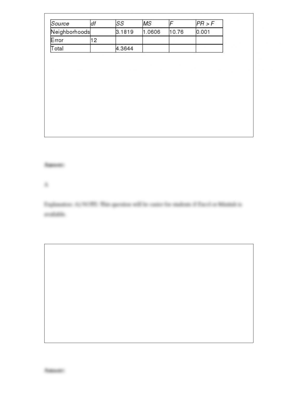
Referring to Table 11-2, the value of the test statistic for Levene’s test for homogeneity
of variances is
A) 0.25.
B) 0.37.
C) 4.36.
D) 10.76.
A university dean is interested in determining the proportion of students who receive
some sort of financial aid. Rather than examine the records for all students, the dean
randomly selects 200 students and finds that 118 of them are receiving financial aid. If
the dean wanted to estimate the proportion of all students receiving financial aid to
within 3% with 99% reliability, how many students would need to be sampled?
A) n = 1,844
B) n = 1,784
C) n = 1,503
D) n = 1,435
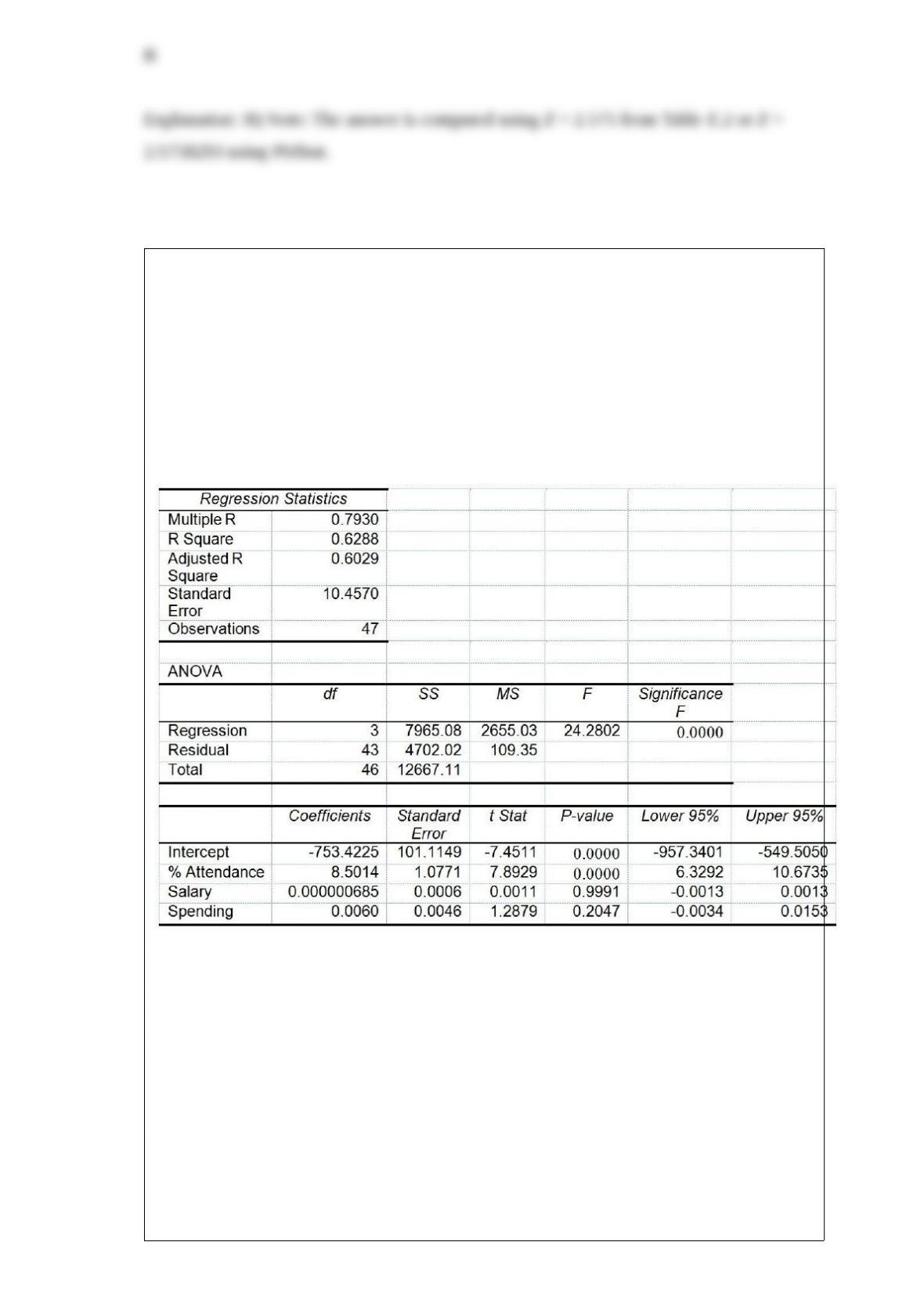
TABLE 17-8
The superintendent of a school district wanted to predict the percentage of students
passing a sixth-grade proficiency test. She obtained the data on percentage of students
passing the proficiency test (% Passing), daily mean of the percentage of students
attending class (% Attendance), mean teacher salary in dollars (Salaries), and
instructional spending per pupil in dollars (Spending) of 47 schools in the state.
Following is the multiple regression output with Y = % Passing as the dependent
variable, X1 = % Attendance, X2 = Salaries and X3 = Spending:
Referring to Table 17-8, which of the following is a correct statement?
A) 60.29% of the total variation in the percentage of students passing the proficiency
test can be explained by daily mean of the percentage of students attending class, mean
teacher salary, and instructional spending per pupil.
B) 60.29% of the total variation in the percentage of students passing the proficiency
test can be explained by daily mean of the percentage of students attending class, mean
teacher salary, and instructional spending per pupil after adjusting for the number of
predictors and sample size.
C) 60.29% of the total variation in the percentage of students passing the proficiency
test can be explained by daily mean of the percentage of students attending class
holding constant the effect of mean teacher salary, and instructional spending per pupil.
D) 60.29% of the total variation in the percentage of students passing the proficiency
test can be explained by daily mean of the percentage of students attending class after
adjusting for the effect of mean teacher salary, and instructional spending per pupil.
TABLE 16-12
A local store developed a multiplicative time-series model to forecast its revenues in
future quarters, using quarterly data on its revenues during the 5-year period from 2008
to 2012. The following is the resulting regression equation:
log10 = 6.102 + 0.012 X – 0.129 1 – 0.054 2 + 0.098 3
where is the estimated number of contracts in a quarter
X is the coded quarterly value with X = 0 in the first quarter of 2008
1 is a dummy variable equal to 1 in the first quarter of a year and 0 otherwise
2 is a dummy variable equal to 1 in the second quarter of a year and 0 otherwise
is a dummy variable equal to 1 in the third quarter of a year and 0 otherwise
Referring to Table 16-12, the estimated quarterly compound growth rate in revenues is
around
A) 1.2%.
B) 2.8%.
C) 12%.
D) 28%.
Which of the following is true regarding the sampling distribution of the mean for a
large sample size?
A) It has the same shape, mean, and standard deviation as the population.
B) It has a normal distribution with the same mean and standard deviation as the
population.
C) It has the same shape and mean as the population, but has a smaller standard

deviation.
D) It has a normal distribution with the same mean as the population but with a smaller
standard deviation.
TABLE 6-5
A company producing orange juice buys all of its oranges from a large orange orchard.
The amount of juice that can be squeezed from each of these oranges is approximately
normally distributed with a mean of 4.7 ounces and some unknown standard deviation.
The company’s production manager knows that the probability is 30.85% that a
randomly selected orange will contain less than 4.5 ounces of juice. Also, the
probability is 10.56% that a randomly selected orange will contain more than 5.2
ounces of juice. Answer the following questions without the help of a calculator,
statistical software or statistical table.
Referring to Table 6-5, what is the probability that a randomly selected orange will
contain between 4.2 and 4.9 ounces of juice?
TABLE 2-8
The Stem-and-Leaf display represents the number of times in a year that a random
sample of 100 “lifetime” members of a health club actually visited the facility.
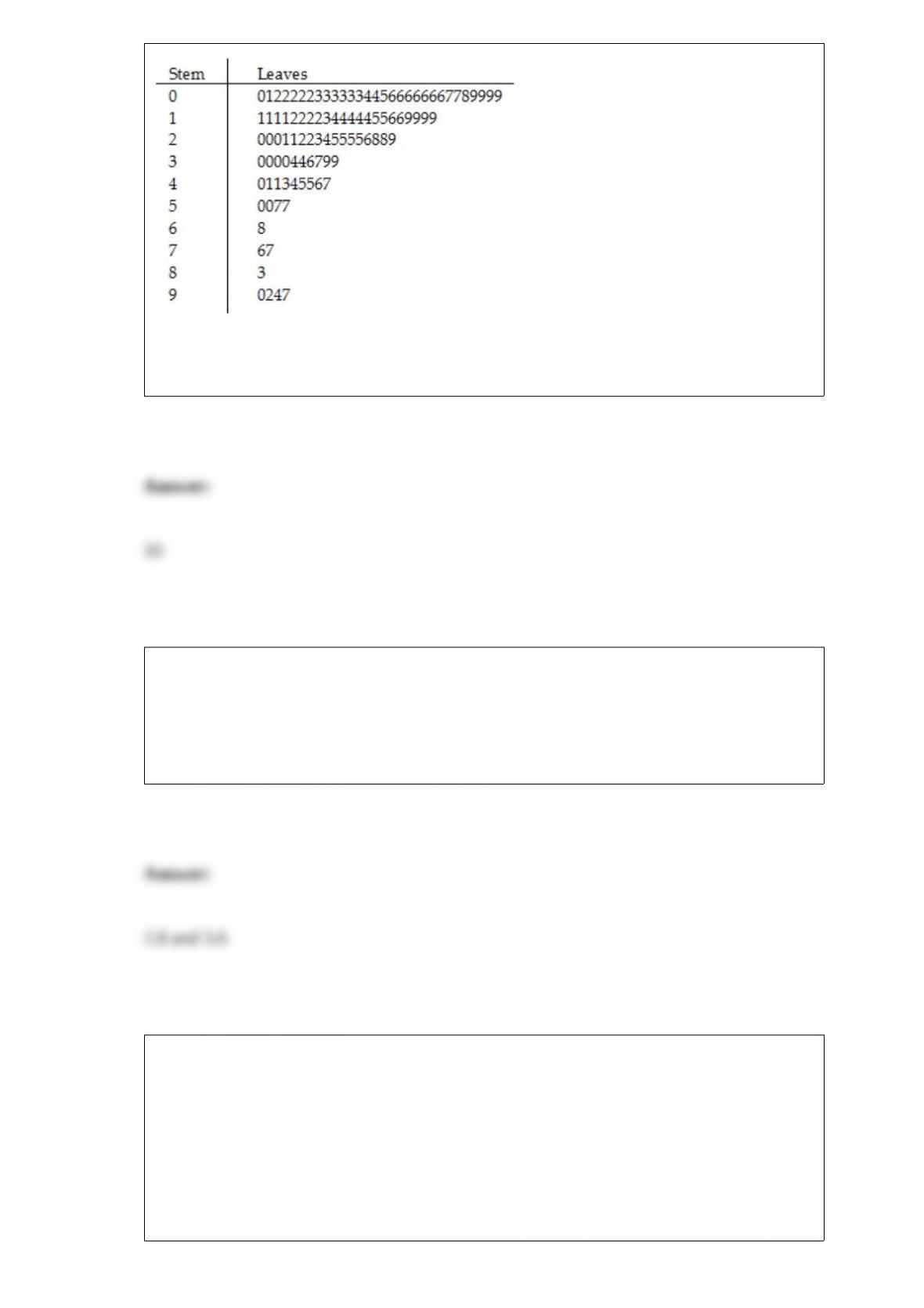
Referring to Table 2-8, ________ of the 100 members visited the health club at least 52
times in a year.
The owner of a fish market determined that the average weight for a catfish is 3.2
pounds. He also knew that the probability of a randomly selected catfish that would
weigh more than 3.8 pounds is 20% and the probability that a randomly selected catfish
that would weigh less than 2.8 pounds is 30%. The middle 40% of the catfish will
weigh between ________ pounds and ________ pounds.
TABLE 17-10
Given below are results from the regression analysis where the dependent variable is
the number of weeks a worker is unemployed due to a layoff (Unemploy) and the
independent variables are the age of the worker (Age), the number of years of education
received (Edu), the number of years at the previous job (Job Yr), a dummy variable for
marital status (Married: 1 = married, 0 = otherwise), a dummy variable for head of
household (Head: 1 = yes, 0 = no) and a dummy variable for management position
(Manager: 1 = yes, 0 = no). We shall call this Model 1. The coefficient of partial

determination ( ) of each of the 6 predictors are, respectively,
0.2807, 0.0386, 0.0317, 0.0141, 0.0958, and 0.1201.
Model 2 is the regression analysis where the dependent variable is Unemploy and the
independent variables are Age and Manager. The results of the regression analysis are
given below:
Referring to Table 17-10 and using both Model 1 and Model 2, what is the p-value of
the test statistic for testing whether the independent variables that are not significant
individually are also not significant as a group in explaining the variation in the
dependent variable at a 5% level of significance?

TABLE 7-6
Online customer service is a key element to successful online retailing. According to a
marketing survey, 37.5% of online customers take advantage of the online customer
service. Random samples of 200 customers are selected.
Referring to Table 7-6, the population mean of all possible sample proportions is
________.
TABLE 17-9
What are the factors that determine the acceleration time (in sec.) from 0 to 60 miles per
hour of a car? Data on the following variables for 171 different vehicle models were
collected:
Accel Time: Acceleration time in sec.
Cargo Vol: Cargo volume in cu. ft.
HP: Horsepower
MPG: Miles per gallon
SUV: 1 if the vehicle model is an SUV with Coupe as the base when SUV and Sedan
are both 0
Sedan: 1 if the vehicle model is a sedan with Coupe as the base when SUV and Sedan
are both 0
The regression results using acceleration time as the dependent variable and the
remaining variables as the independent variables are presented below.
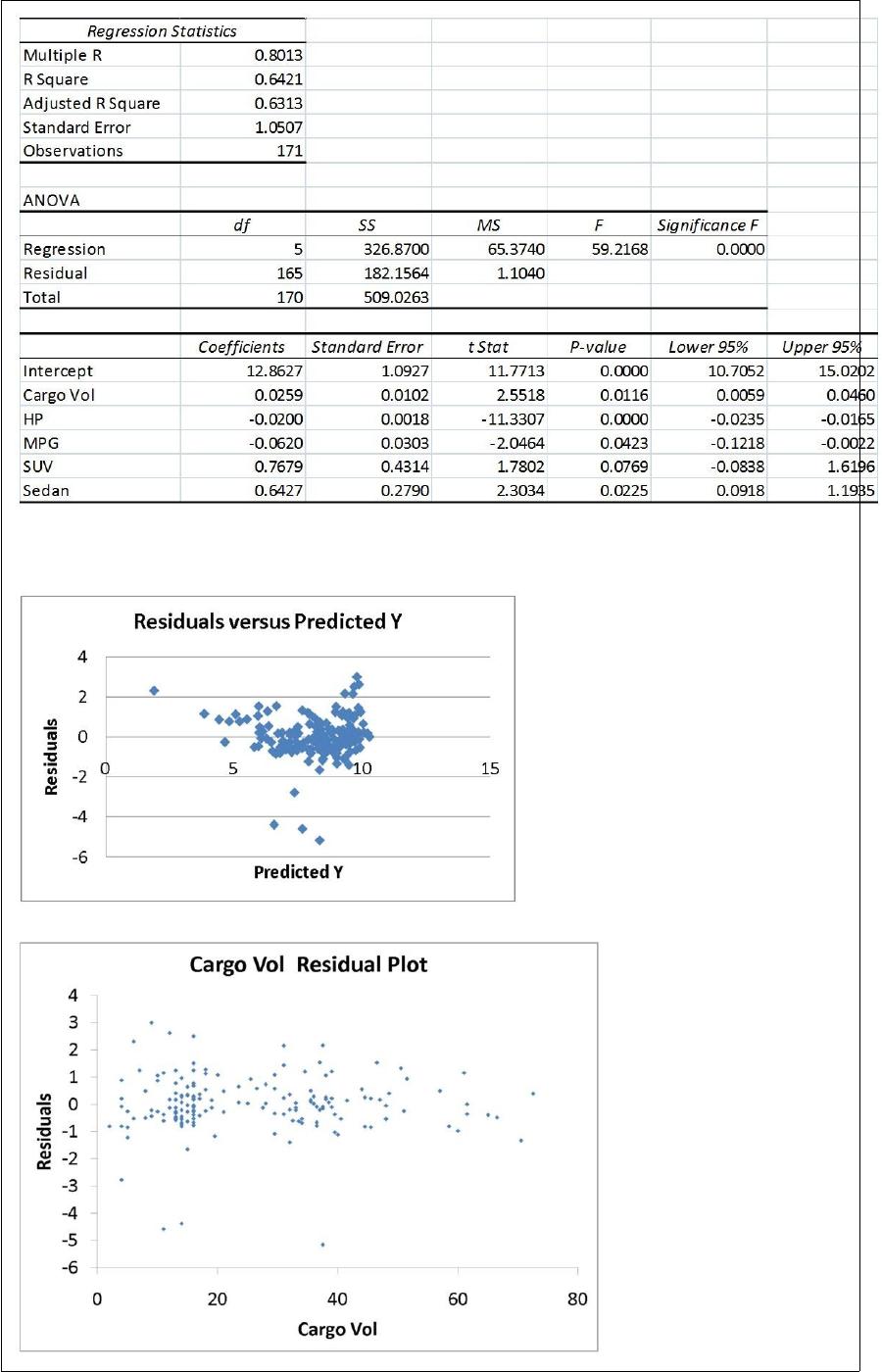
The various residual plots are as shown below.
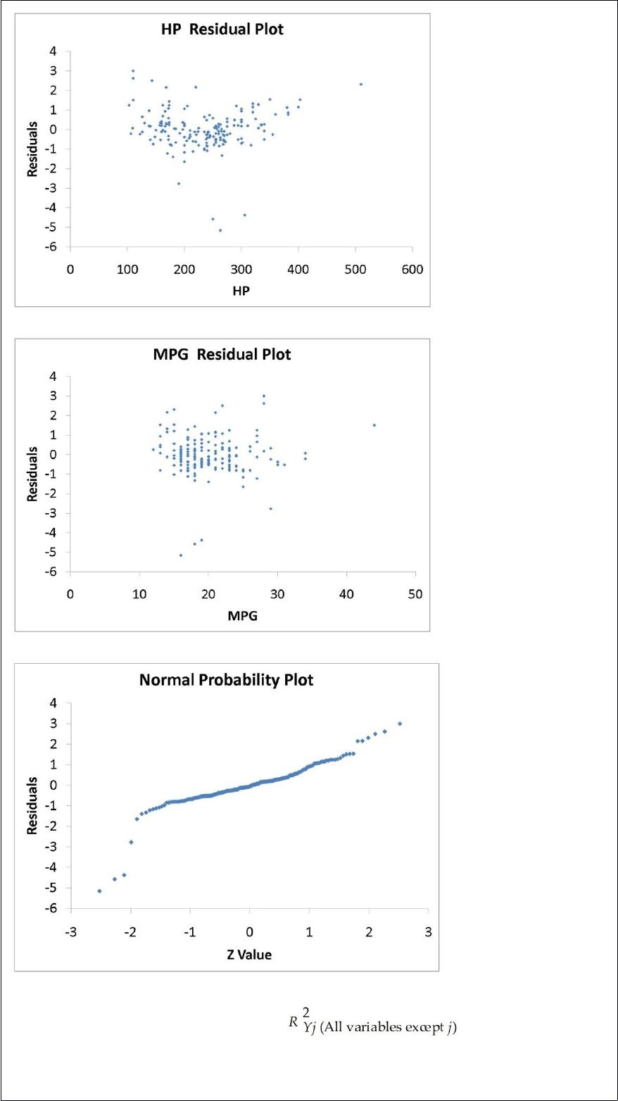
The coefficient of partial determination ( ) of each of the 5
predictors are, respectively, 0.0380, 0.4376, 0.0248, 0.0188, and 0.0312.

The coefficient of multiple determination for the regression model using each of the 5
variables Xj as the dependent variable and all other X variables as independent variables
( ) are, respectively, 0.7461, 0.5676, 0.6764, 0.8582, 0.6632.
Referring to Table 17-9, what is the p-value of the test statistic to determine whether
SUV makes a significant contribution to the regression model in the presence of the
other independent variables at a 5% level of significance?
Referring to Table 14-17, what is the value of the test statistic when
testing whether age has any effect on the number of weeks a worker
is unemployed due to a layoff while holding constant the effect of the
other independent variable?
TABLE 14-17
Given below are results from the regression analysis where the
dependent variable is the number of weeks a worker is unemployed
due to a layoff (Unemploy) and the independent variables are the age
of the worker (Age) and a dummy variable for management position
(Manager: 1 = yes, 0 = no).
The results of the regression analysis are given below: