
TABLE 9-1
Microsoft Excel was used on a set of data involving the number of defective items
found in a random sample of 46 cases of light bulbs produced during a morning shift at
a plant. A manager wants to know if the mean number of defective bulbs per case is
greater than 20 during the morning shift. She will make her decision using a test with a
level of significance of 0.10. The following information was extracted from the
Microsoft Excel output for the sample of 46 cases:
True or False: Referring to Table 9-1, the null hypothesis would be rejected if a 5%
probability of committing a Type I error is allowed.
True or False: An ogive is a cumulative percentage polygon.
True or False: Given a data set with 15 yearly observations, there are only thirteen
3-year moving averages.
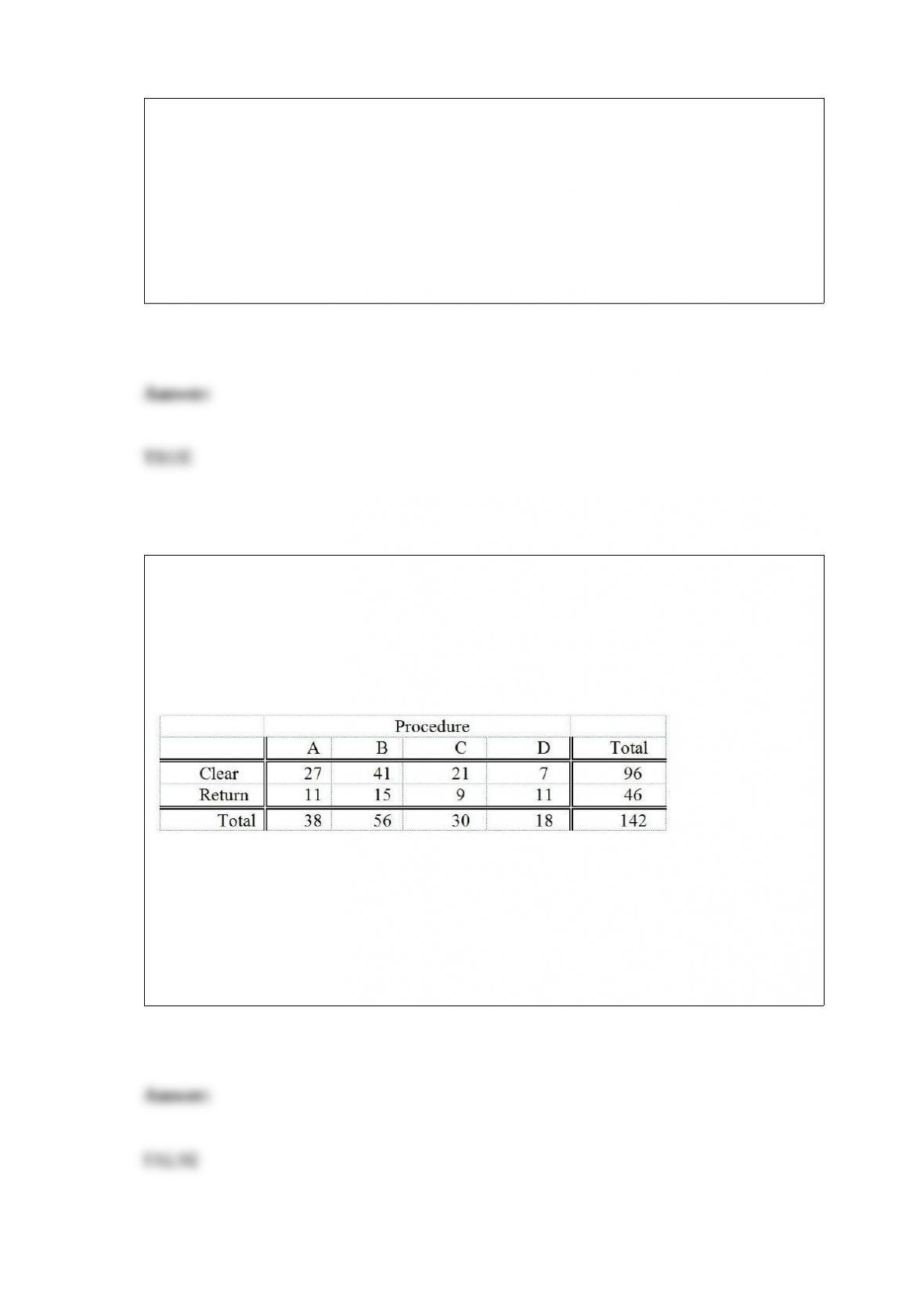
TABLE 8-8
The president of a university would like to estimate the proportion of the student
population that owns a personal computer. In a sample of 500 students, 417 own a
personal computer.
True or False: Referring to Table 8-8, the parameter of interest is the proportion of the
student population who own a personal computer.
TABLE 12-5
Four surgical procedures currently are used to install pacemakers. If the patient does not
need to return for follow-up surgery, the operation is called a “clear” operation. A heart
center wants to compare the proportion of clear operations for the 4 procedures, and
collects the following numbers of patients from their own records:
They will use this information to test for a difference among the proportion of clear
operations using a chi-square test with a level of significance of 0.05.
True or False: Referring to Table 12-5, there is sufficient evidence to conclude that the
proportions between procedure B and procedure D are different at a 0.05 level of
significance.

True or False: When the parametric assumption on the distribution is met, a parametric
test is usually more powerful than a nonparametric test.
True or False: Given a data set with 15 yearly observations, a 3-year moving average
will have fewer observations than a 5-year moving average.
TABLE 9-3
An appliance manufacturer claims to have developed a compact microwave oven that
consumes a mean of no more than 250 W. From previous studies, it is believed that
power consumption for microwave ovens is normally distributed with a population
standard deviation of 15 W. A consumer group has decided to try to discover if the
claim appears true. They take a sample of 20 microwave ovens and find that they
consume a mean of 257.3 W.
Referring to Table 9-3, the appropriate hypotheses to determine if the manufacturer’s
claim appears reasonable are
A) H0 : = 250 versus H1 : ≠250.
B) H0 : 250 versus H1 : < 250.
C) H0 : 250 versus H1 : > 250.
D) H0 : 257.3 versus H1 : < 257.3.
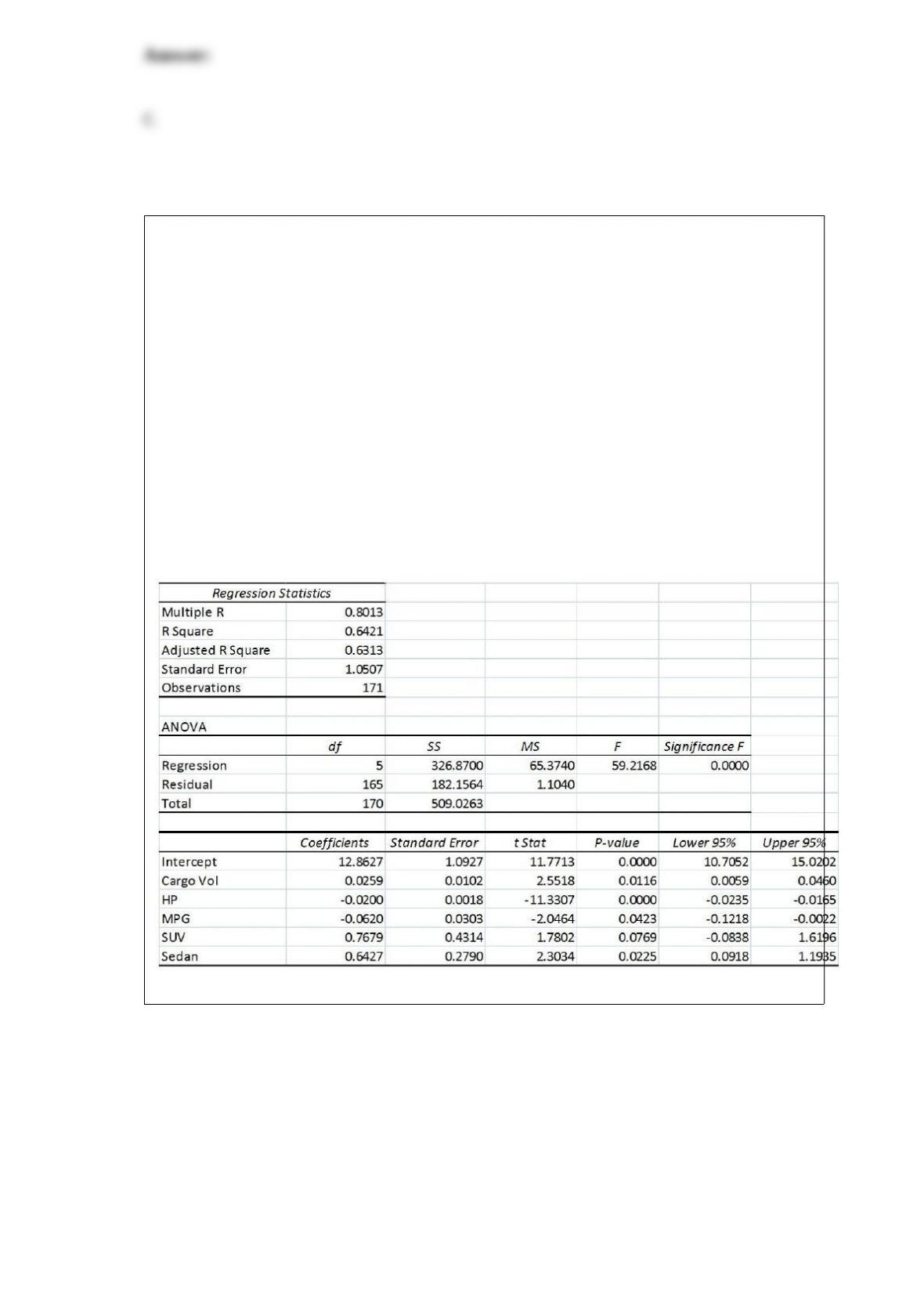
TABLE 17-9
What are the factors that determine the acceleration time (in sec.) from 0 to 60 miles per
hour of a car? Data on the following variables for 171 different vehicle models were
collected:
Accel Time: Acceleration time in sec.
Cargo Vol: Cargo volume in cu. ft.
HP: Horsepower
MPG: Miles per gallon
SUV: 1 if the vehicle model is an SUV with Coupe as the base when SUV and Sedan
are both 0
Sedan: 1 if the vehicle model is a sedan with Coupe as the base when SUV and Sedan
are both 0
The regression results using acceleration time as the dependent variable and the
remaining variables as the independent variables are presented below.
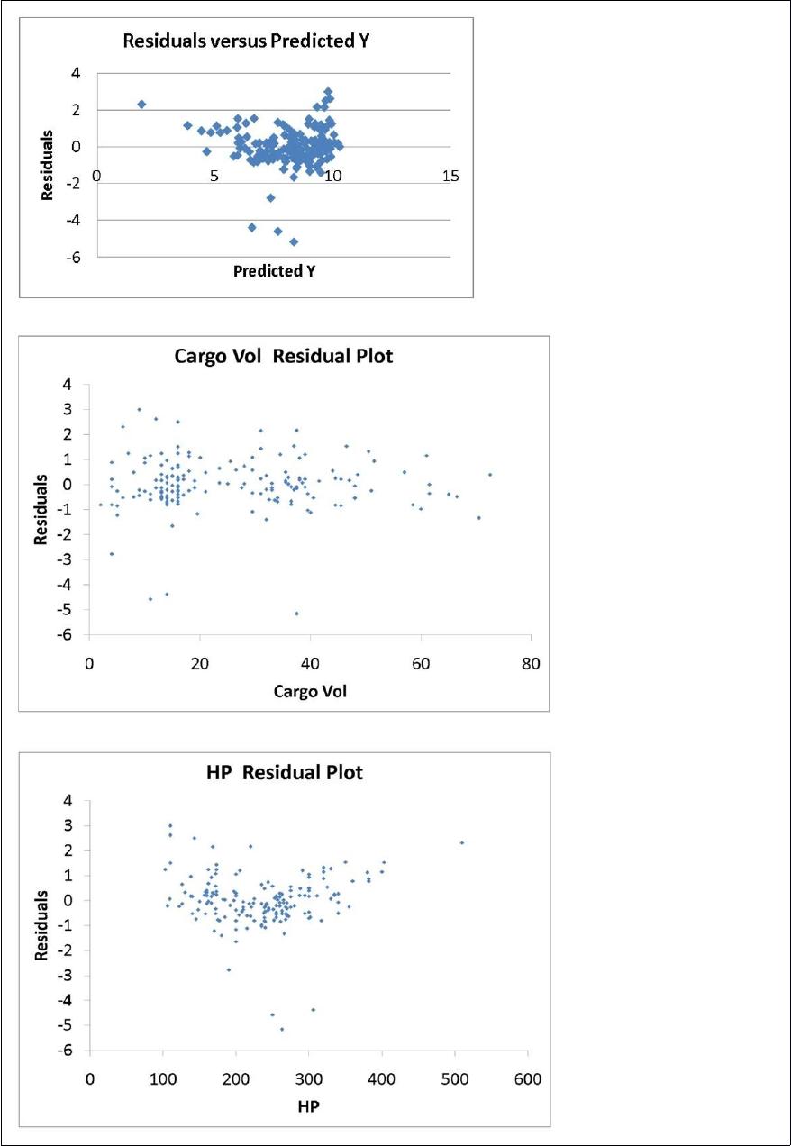
The various residual plots are as shown below.
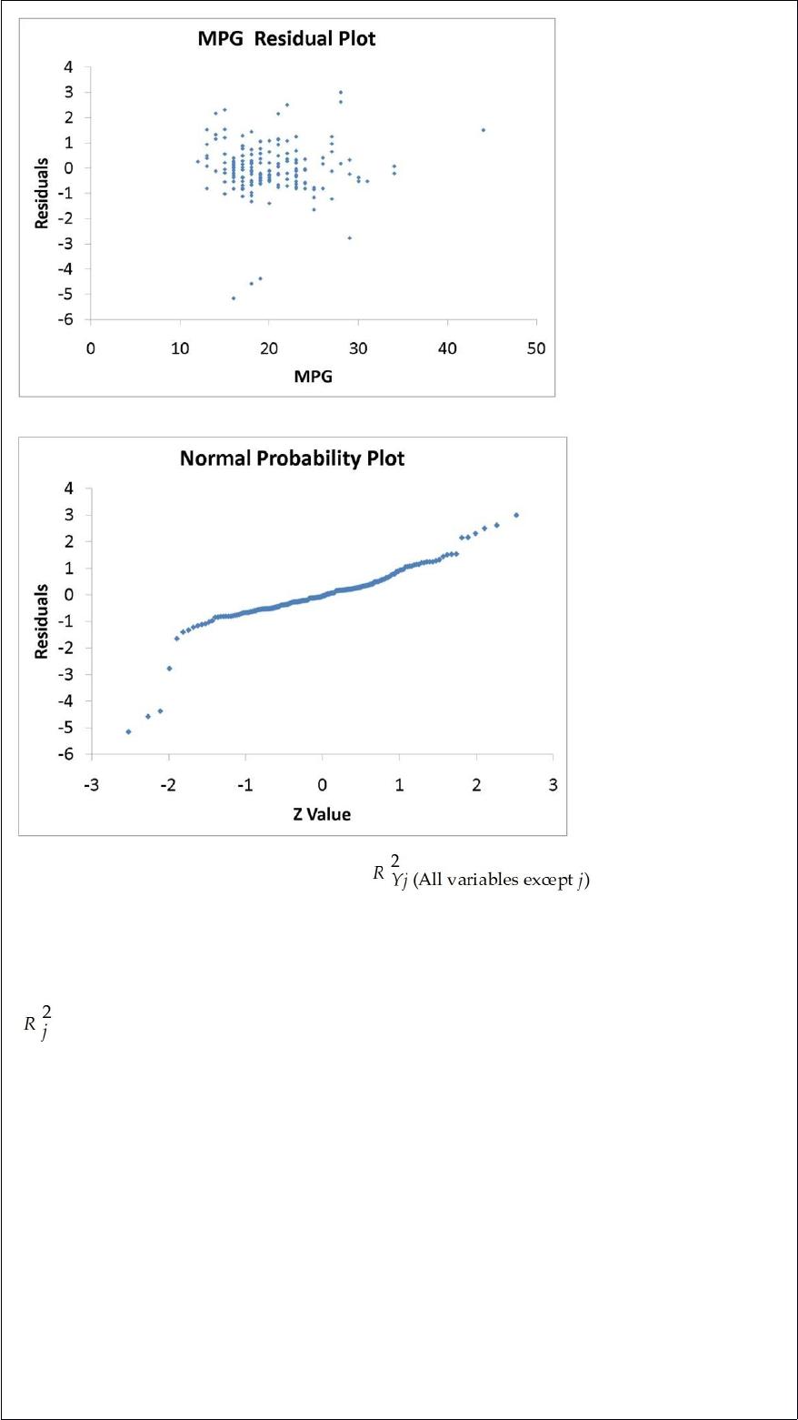
The coefficient of partial determination ( ) of each of the 5
predictors are, respectively, 0.0380, 0.4376, 0.0248, 0.0188, and 0.0312.
The coefficient of multiple determination for the regression model using each of the 5
variables Xj as the dependent variable and all other X variables as independent variables
( ) are, respectively, 0.7461, 0.5676, 0.6764, 0.8582, 0.6632.
Referring to Table 17-9, what is the correct interpretation for the estimated coefficient
for MPG?
A) As the miles per gallon decreases by one unit, the mean 0 to 60 miles per hour
acceleration time will increase by an estimated 0.0620 seconds without taking into
consideration all the other independent variables included in the model.
B) As the 0 to 60 miles per hour acceleration time decreases by one second, the mean
miles per gallon will increase by an estimated 0.0620 unit without taking into
consideration all the other independent variables included in the model.
C) As the miles per gallon decreases by one unit, the mean 0 to 60 miles per hour
acceleration time will increase by an estimated 0.0620 seconds taking into
consideration all the other independent variables included in the model.
D) As the 0 to 60 miles per hour acceleration time decreases by one second, the mean
miles per gallon will increase by an estimated 0.0620 unit taking into consideration all
the other independent variables included in the model.
TABLE 17-7
As a project for his business statistics class, a student examined the factors that
determined parking meter rates throughout the campus area. Data were collected for the
price per hour of parking, blocks to the quadrangle, and one of the three jurisdictions:
on campus, in downtown and off campus, or outside of downtown and off campus. The
population regression model hypothesized is
Yi= α + β1X1i + β2X2i + β3X3i + ε
where
Y is the meter price
X1 is the number of blocks to the quad
X2 is a dummy variable that takes the value 1 if the meter is located in downtown and
off campus and the value 0 otherwise
X3 is a dummy variable that takes the value 1 if the meter is located outside of
downtown and off campus, and the value 0 otherwise
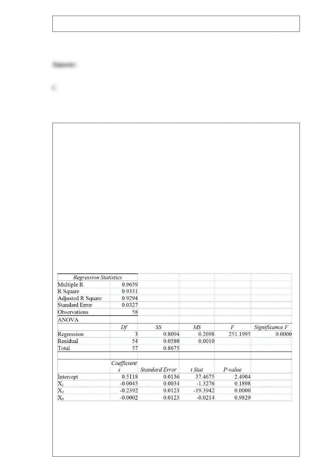
The following Excel results are obtained.
Referring to Table 17-7, if one is already outside of downtown and off campus but
decides to park 3 more blocks from the quad, the estimated mean parking meter rate
will
A) decrease by 0.0045.
B) decrease by 0.0135.
C) decrease by 0.0139.
D) decrease by 0.4979.
TABLE 17-2
One of the most common questions of prospective house buyers pertains to the cost of
heating in dollars (Y). To provide its customers with information on that matter, a large
real estate firm used the following 4 variables to predict heating costs: the daily
minimum outside temperature in degrees of Fahrenheit (X1), the amount of insulation in
inches (X2), the number of windows in the house (X3), and the age of the furnace in
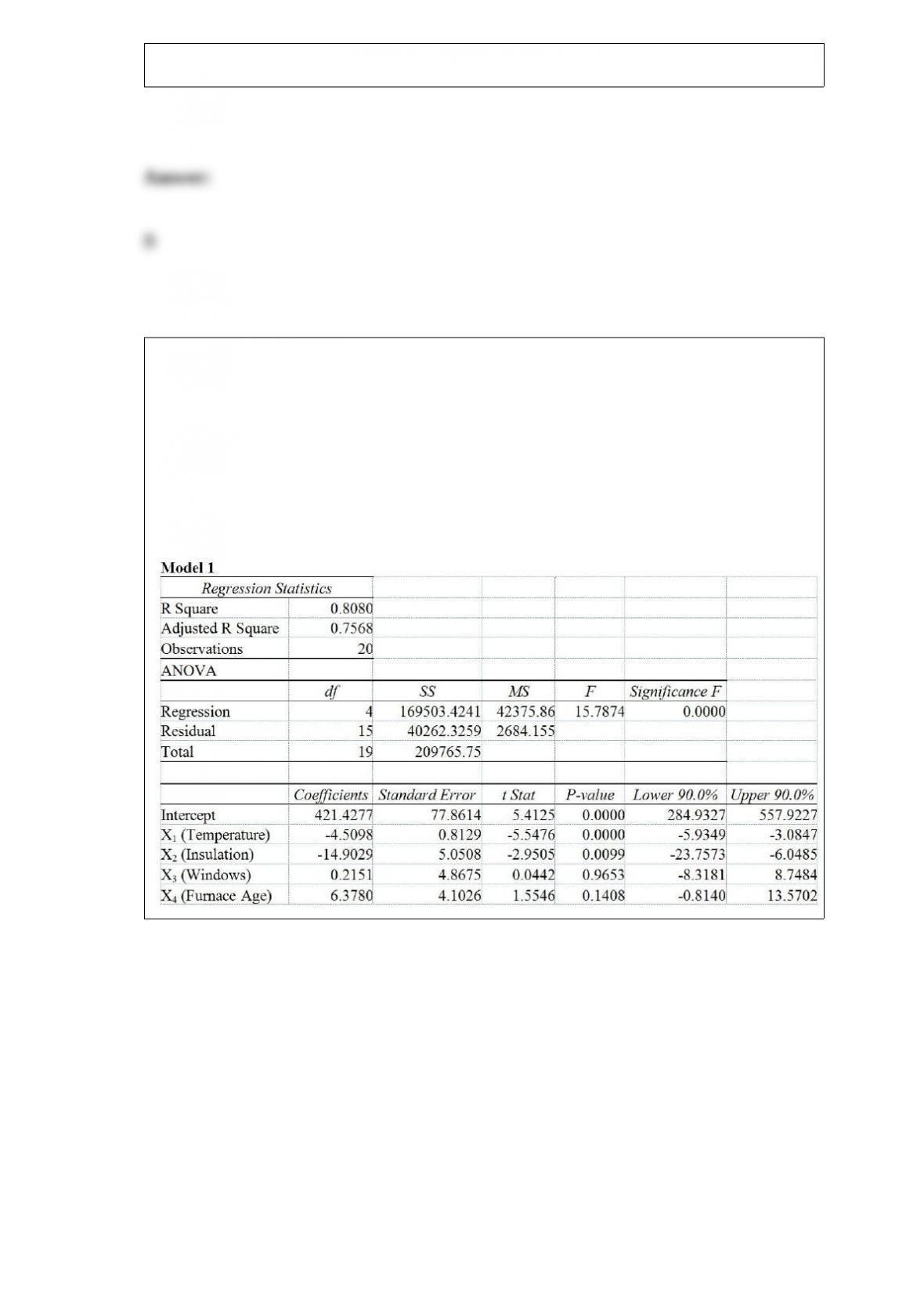
years (X4). Given below are the EXCEL outputs of two regression models.

Referring to Table 17-2, the estimated value of the partial regression parameter β1in
Model 1 means that
A) holding the effect of the other independent variables constant, an estimated expected
$1 increase in heating costs is associated with a decrease in the daily minimum outside
temperature by 4.51 degrees.
B) holding the effect of the other independent variables constant, a 1 degree increase in
the daily minimum outside temperature results in a decrease in heating costs by $4.51.
C) holding the effect of the other independent variables constant, a 1 degree increase in
the daily minimum outside temperature results in an estimated decrease in mean heating
costs by $4.51.
D) holding the effect of the other independent variables constant, a 1% increase in the
daily minimum outside temperature results in an estimated decrease in mean heating
costs by 4.51%.
TABLE 9-2
A student claims that he can correctly identify whether a person is a business major or
an agriculture major by the way the person dresses. Suppose in actuality that if someone
is a business major, he can correctly identify that person as a business major 87% of the
time. When a person is an agriculture major, the student will incorrectly identify that
person as a business major 16% of the time. Presented with one person and asked to
identify the major of this person (who is either a business or an agriculture major), he
considers this to be a hypothesis test with the null hypothesis being that the person is a
business major and the alternative that the person is an agriculture major.
Referring to Table 9-2, what is the power of the test?

A) 0.13
B) 0.16
C) 0.84
D) 0.87
The probability that house sales will increase in the next 6 months is estimated to be
0.25. The probability that the interest rates on housing loans will go up in the same
period is estimated to be 0.74. The probability that house sales or interest rates will go
up during the next 6 months is estimated to be 0.89. The events increase in house sales
and no increase in house sales in the next 6 months are
A) independent.
B) mutually exclusive.
C) collectively exhaustive.
D) B and C.
The local police department must write, on average, 5 tickets a day to keep department
revenues at budgeted levels. Suppose the number of tickets written per day follows a
Poisson distribution with a mean of 6.5 tickets per day. Interpret the value of the mean.
A) The number of tickets that is written most often is 6.5 tickets per day.
B) Half of the days have less than 6.5 tickets written and half of the days have more
than 6.5 tickets written.
C) If we sampled all days, the arithmetic average or expected number of tickets written
would be 6.5 tickets per day.
D) The mean has no interpretation since 0.5 ticket can never be written.
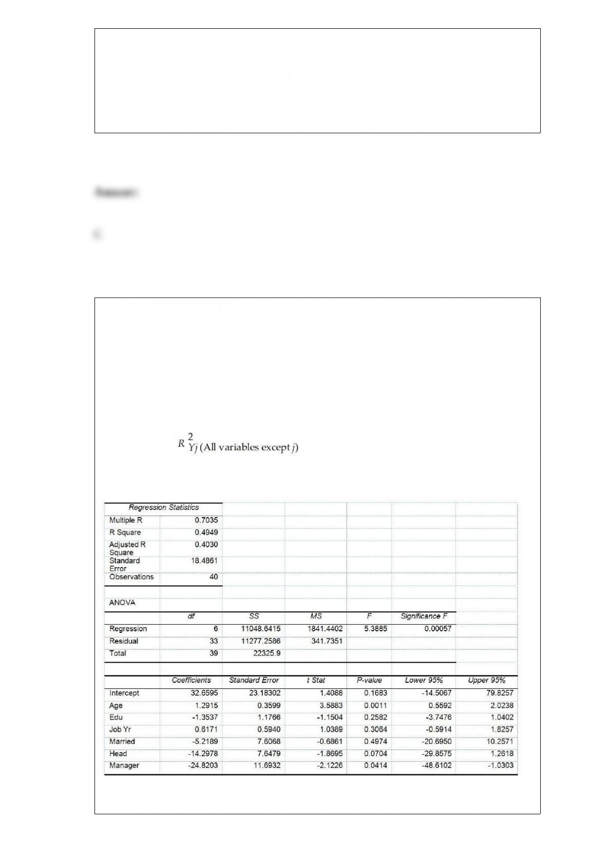
TABLE 17-10
Given below are results from the regression analysis where the dependent variable is
the number of weeks a worker is unemployed due to a layoff (Unemploy) and the
independent variables are the age of the worker (Age), the number of years of education
received (Edu), the number of years at the previous job (Job Yr), a dummy variable for
marital status (Married: 1 = married, 0 = otherwise), a dummy variable for head of
household (Head: 1 = yes, 0 = no) and a dummy variable for management position
(Manager: 1 = yes, 0 = no). We shall call this Model 1. The coefficient of partial
determination ( ) of each of the 6 predictors are, respectively,
0.2807, 0.0386, 0.0317, 0.0141, 0.0958, and 0.1201.
Model 2 is the regression analysis where the dependent variable is Unemploy and the
independent variables are Age and Manager. The results of the regression analysis are
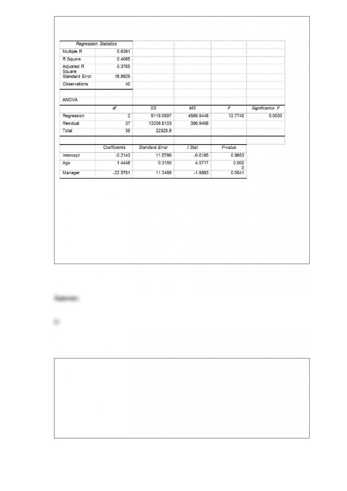
given below:
Referring to Table 17-10, Model 1, which of the following is the correct alternative
hypothesis to test whether being married or not makes a difference in the mean number
of weeks a worker is unemployed due to a layoff while holding constant the effect of all
the other independent variables?
A) H1 : β1 ≠0
B) H1 : β2 ≠0
C) H1 : β3 ≠0
D) H1 : β4 ≠0
TABLE 17-8
The superintendent of a school district wanted to predict the percentage of students
passing a sixth-grade proficiency test. She obtained the data on percentage of students
passing the proficiency test (% Passing), daily mean of the percentage of students
attending class (% Attendance), mean teacher salary in dollars (Salaries), and
instructional spending per pupil in dollars (Spending) of 47 schools in the state.
Following is the multiple regression output with Y = % Passing as the dependent
variable, X1 = % Attendance, X2 = Salaries and X3 = Spending:
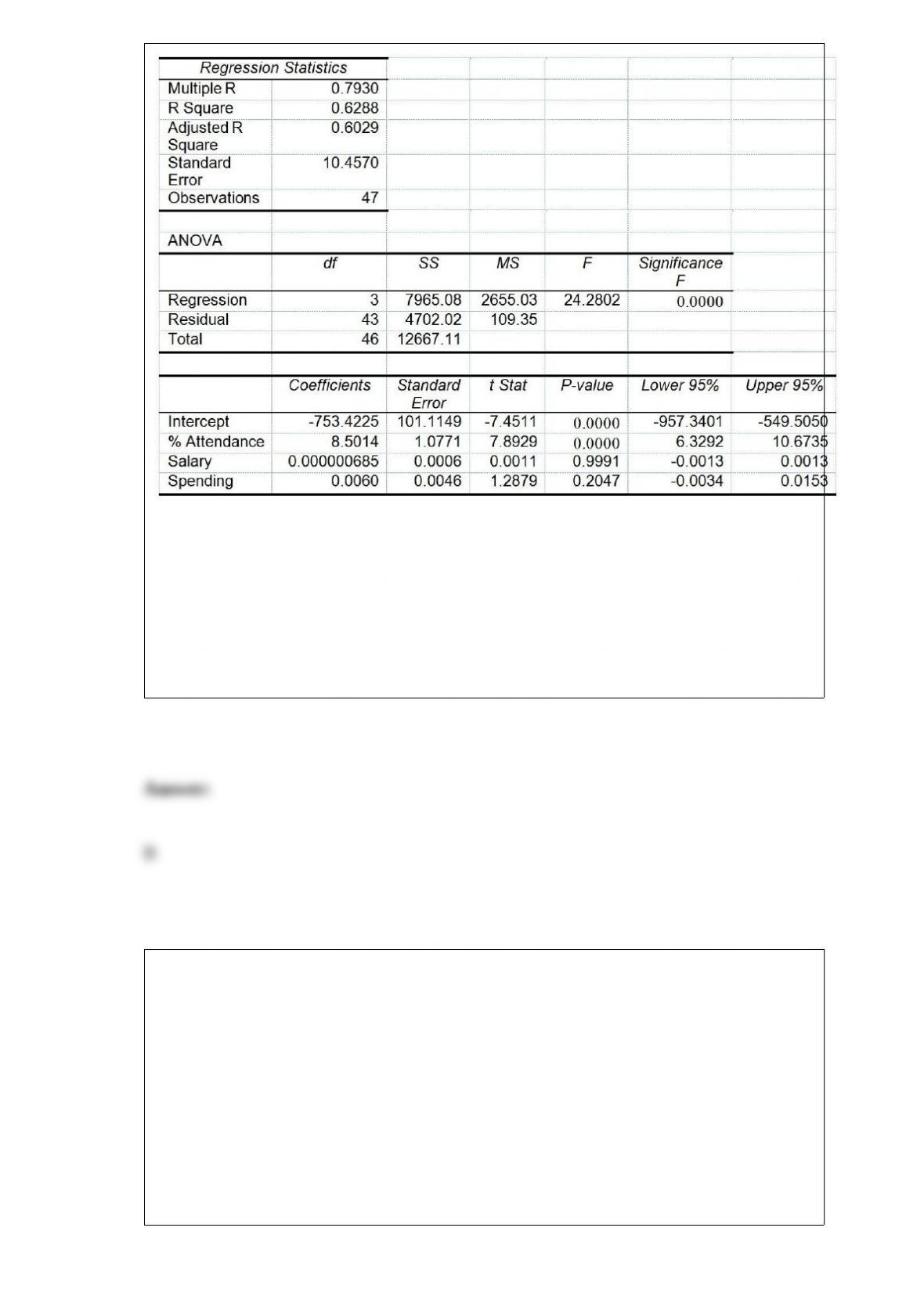
Referring to Table 17-8, which of the following is the correct null hypothesis to
determine whether there is a significant relationship between the percentage of students
passing the proficiency test and the entire set of explanatory variables?
A) H0 : β0 = β1 = β2 = β3 = 0
B) H0 : β1 = β2 = β3 = 0
C) H0 : β0 = β1 = β2 = β3 ≠0
D) H0 : β1 = β2 = β3 ≠0
One of the developing countries is experiencing a baby boom, with the number of births
rising for the fifth year in a row, according to a BBC News report. Which of the
following is best for displaying this data?
A) A Pareto chart
B) A two-way classification table
C) A histogram
D) A time-series plot

For a potential investment of $5,000, a portfolio has an EMV of $1,000 and a standard
deviation of $100. What is the rate of return?
A) 5%
B) 10%
C) 20%
D) 50%
The probability that a new advertising campaign will increase sales is assessed as being
0.80. The probability that the cost of developing the new ad campaign can be kept
within the original budget allocation is 0.40. Assuming that the two events are
independent, the probability that the cost is kept within budget or the campaign will
increase sales is
A) 0.20.
B) 0.32.
C) 0.68.
D) 0.88.

The sample correlation coefficient between X and Y is 0.375. It has been found out that
the p-value is 0.256 when testing H0 : = 0 against the two-sided alternative H1 :
0. To test H0 : = 0 against the one-sided alternative H1 : > 0 at a significance level of
0.1, the p-value is
A) 0.256 / 2.
B) (0.256) 2.
C) 1 – 0.256.
D) 1 – 0.256 / 2.
An agronomist wants to compare the crop yield of 3 varieties of chickpea seeds. She
plants all 3 varieties of the seeds on each of 5 different patches of fields. She then
measures the crop yield in bushels per acre. Which of the following tests will be the
most appropriate to find out if there is any difference in crop yield among the 3
varieties?
A) Randomized block F test for block effect
B) One-way ANOVA F test for differences among more than two means
C) Randomized block F test for differences among more than two means
D) Two-way ANOVA F test for the variety effect
TABLE 19-1
The following payoff table shows profits associated with a set of 3 alternatives under 2

possible states of nature
Referring to Table 19-1, if the probability of S1 is 0.5, then the coefficient of variation
for A2 is
A) 0.231.
B) 0.5.
C) 1.5.
D) 2.
The logarithm transformation can be used
A) to overcome violations to the autocorrelation assumption.
B) to test for possible violations to the autocorrelation assumption.
C) to change a nonlinear model into a linear model.
D) to change a linear independent variable into a nonlinear independent variable.
The Commissioner of Health in New York State wanted to study malpractice litigation
in New York. A sample of 31 thousand medical records was drawn from a population of
2.7 million patients who were discharged during 2010. The collection, presentation, and
characterization of the data from patient medical records are examples of ________.
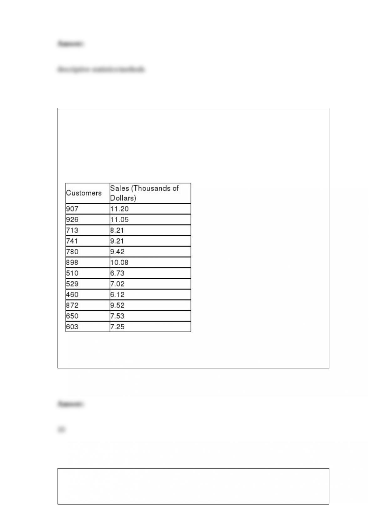
TABLE 13-10
The management of a chain electronic store would like to develop a model for
predicting the weekly sales (in thousands of dollars) for individual stores based on the
number of customers who made purchases. A random sample of 12 stores yields the
following results:
Referring to Table 13-10, what are the degrees of freedom of the t test statistic when
testing whether the number of customers who make a purchase affects weekly sales?
TABLE 13-4
The managers of a brokerage firm are interested in finding out if the number of new
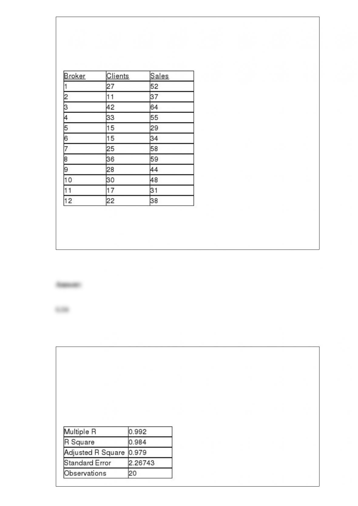
clients a broker brings into the firm affects the sales generated by the broker. They
sample 12 brokers and determine the number of new clients they have enrolled in the
last year and their sales amounts in thousands of dollars. These data are presented in the
table that follows.
Referring to Table 13-4, the managers of the brokerage firm wanted to test the
hypothesis that the population slope was equal to 0. The value of the test statistic is
________.
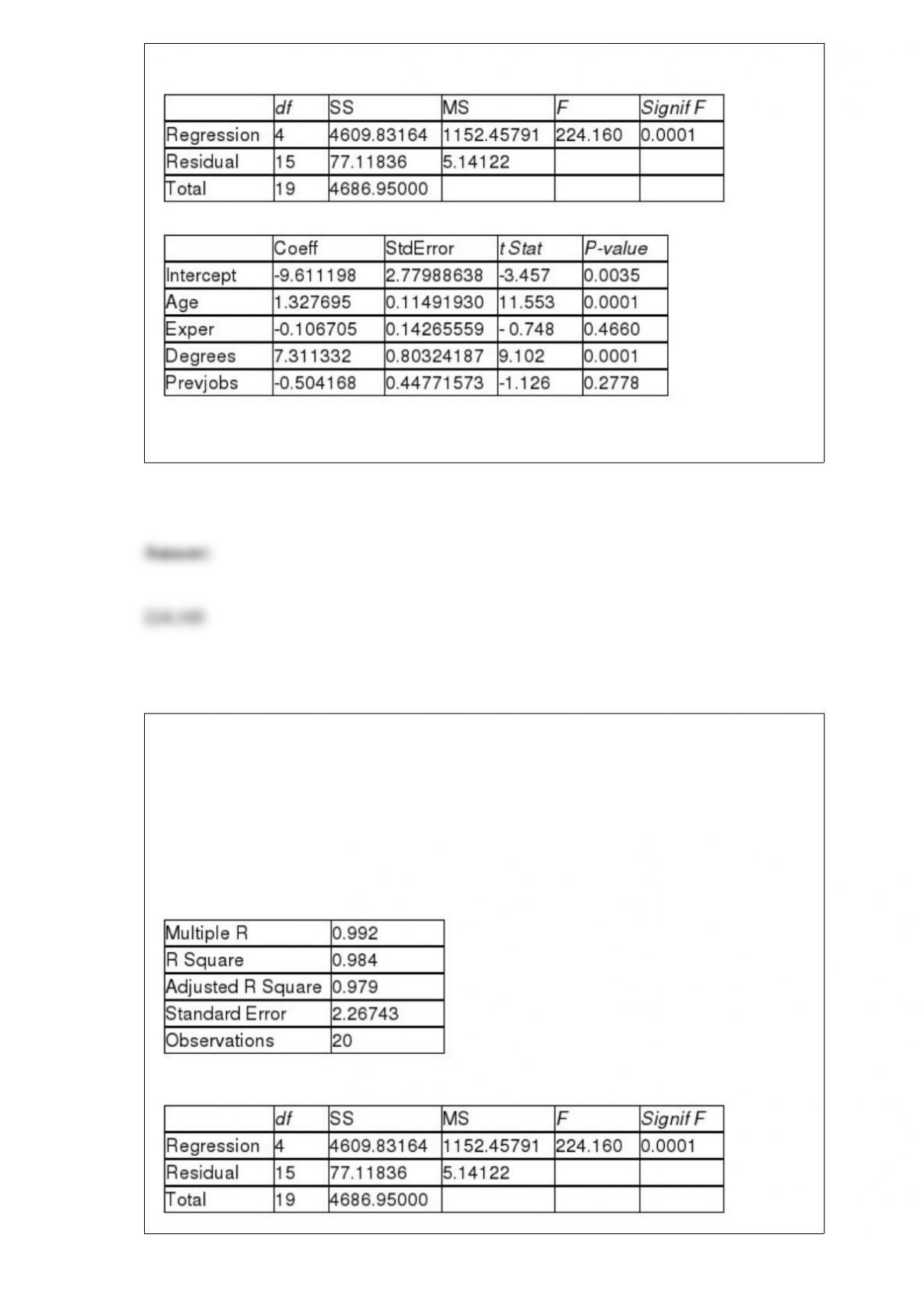
TABLE 17-3
A financial analyst wanted to examine the relationship between salary (in $1,000) and 4
variables: age (X1 = Age), experience in the field (X2 = Exper), number of degrees (X3 =
Degrees), and number of previous jobs in the field (X4 = Prevjobs). He took a sample of
20 employees and obtained the following Microsoft Excel output:
SUMMARY OUTPUT
Regression Statistics
ANOVA
Referring to Table 17-3, the value of the F-statistic for testing the significance of the
entire regression is ________.
TABLE 17-3
A financial analyst wanted to examine the relationship between salary (in $1,000) and 4
variables: age (X1 = Age), experience in the field (X2 = Exper), number of degrees (X3 =
Degrees), and number of previous jobs in the field (X4 = Prevjobs). He took a sample of
20 employees and obtained the following Microsoft Excel output:
SUMMARY OUTPUT
Regression Statistics
ANOVA

Referring to Table 17-3, the p-value of the F test for the significance of the entire
regression is ________.
TABLE 4-3
A survey is taken among customers of a fast-food restaurant to determine preference for
hamburger or chicken. Of 200 respondents selected, 75 were children and 125 were
adults. 120 preferred hamburger and 80 preferred chicken. 55 of the children preferred
hamburger.
Referring to Table 4-3, the probability that a randomly selected individual is an adult or
a child is ________.
TABLE 6-2
John has two jobs. For daytime work at a jewelry store he is paid $15,000 per month,
plus a commission. His monthly commission is normally distributed with a mean of
$10,000 and a standard deviation of $2,000. At night he works occasionally as a waiter,
for which his monthly income is normally distributed with a mean of $1,000 and a
standard deviation of $300. John’s income levels from these two sources are
independent of each other.

Referring to Table 6-2, for a given month, what is the probability that John’s income as
a waiter is no more than $300?