True or False: TABLE 17-3
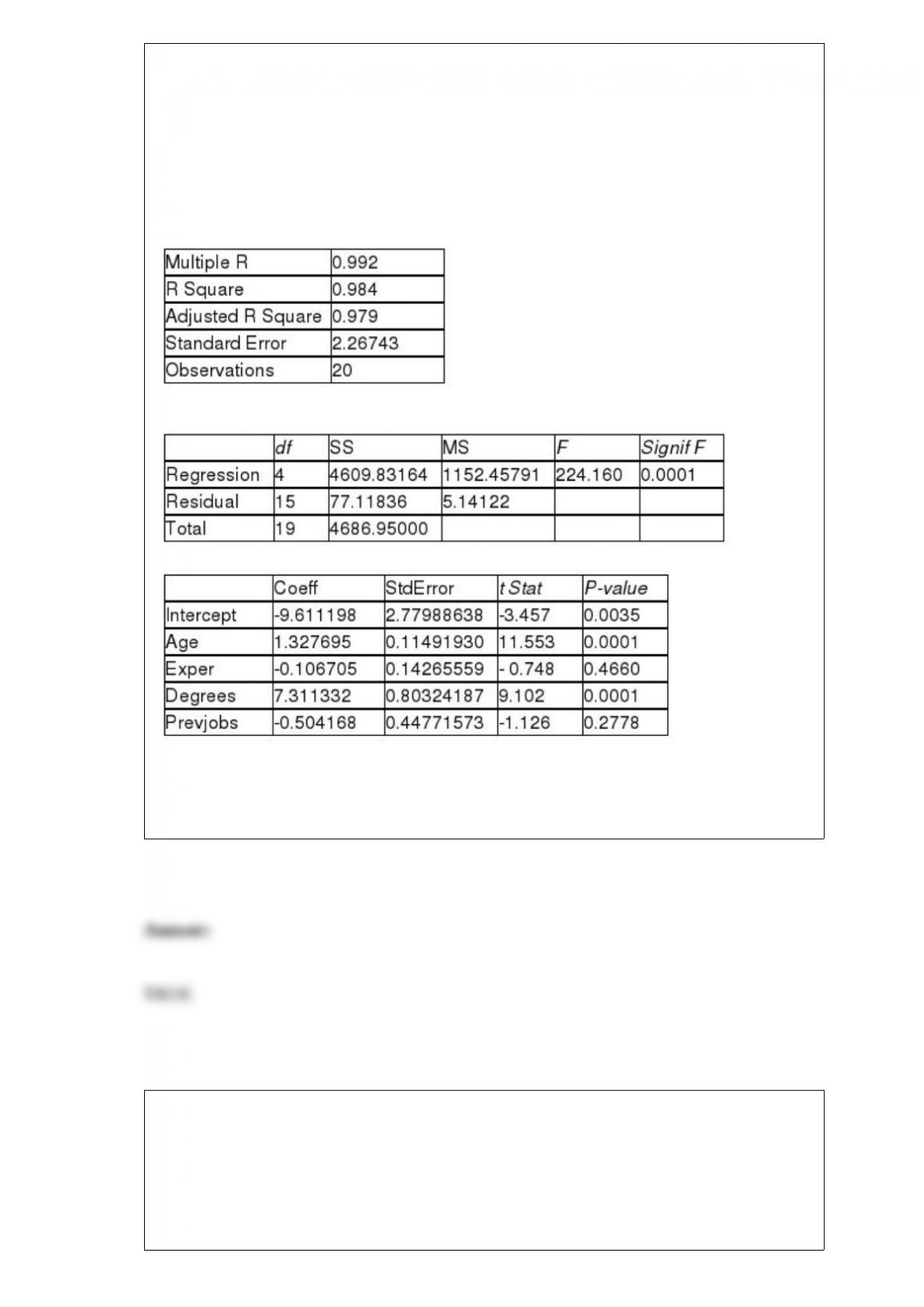
A financial analyst wanted to examine the relationship between salary (in $1,000) and 4
variables: age (X1 = Age), experience in the field (X2 = Exper), number of degrees (X3 =
Degrees), and number of previous jobs in the field (X4 = Prevjobs). He took a sample of
20 employees and obtained the following Microsoft Excel output:
SUMMARY OUTPUT
Regression Statistics
ANOVA
Referring to Table 17-3, the analyst wants to use a t test to test for the significance of
the coefficient of X3. At a level of significance of 0.01, the department head would
decide that β3 ≠0.
TABLE 8-3
To become an actuary, it is necessary to pass a series of 10 exams, including the most
important one, an exam in probability and statistics. An insurance company wants to
estimate the mean score on this exam for actuarial students who have enrolled in a
special study program. They take a sample of 8 actuarial students in this program and
determine that their scores are: 2, 5, 8, 8, 7, 6, 5, and 7. This sample will be used to
calculate a 90% confidence interval for the mean score for actuarial students in the
special study program.
True or False: Referring to Table 8-3, if we use the same sample information to obtain a
95% confidence interval, the resulting interval would be narrower than the one obtained
here with 90% confidence.
TABLE 11-8
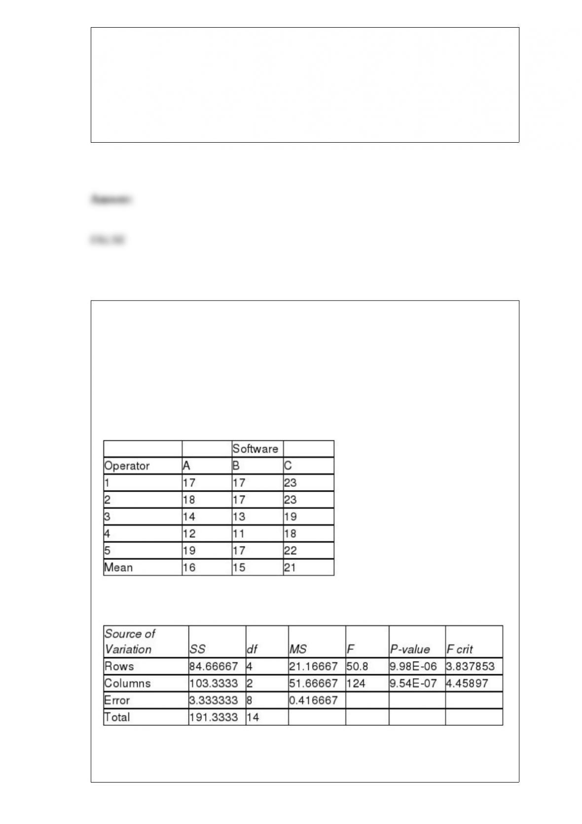
An important factor in selecting database software is the time required for a user to
learn how to use the system. To evaluate three potential brands (A, B and C) of database
software, a company designed a test involving five different employees. To reduce
variability due to differences among employees, each of the five employees is trained
on each of the three different brands. The amount of time (in hours) needed to learn
each of the three different brands is given below:
Below is the Excel output for the randomized block design:
True or False: Referring to Table 11-8, the randomized block F test is valid only if there
is no interaction between the amount of time needed on the 3 brands of software and the

5 employees.
True or False: Suppose, in testing a hypothesis about a mean, the p-value is computed
to be 0.043. The null hypothesis should be rejected if the chosen level of significance is
0.05.
True or False: The variance of the sum of two investments will be equal to the sum of
the variances of the two investments plus twice the covariance between the investments.
TABLE 1-1
The manager of the customer service division of a major consumer electronics company
is interested in determining whether the customers who have purchased a Blu-ray
player made by the company over the past 12 months are satisfied with their products.
Referring to Table 1-1, the possible responses to the question “How many Blu-ray
players made by other manufacturers have you used?” are values from a
A) discrete variable.
B) continuous variable.
C) categorical variable.
D) table of random numbers.
TABLE 13-8
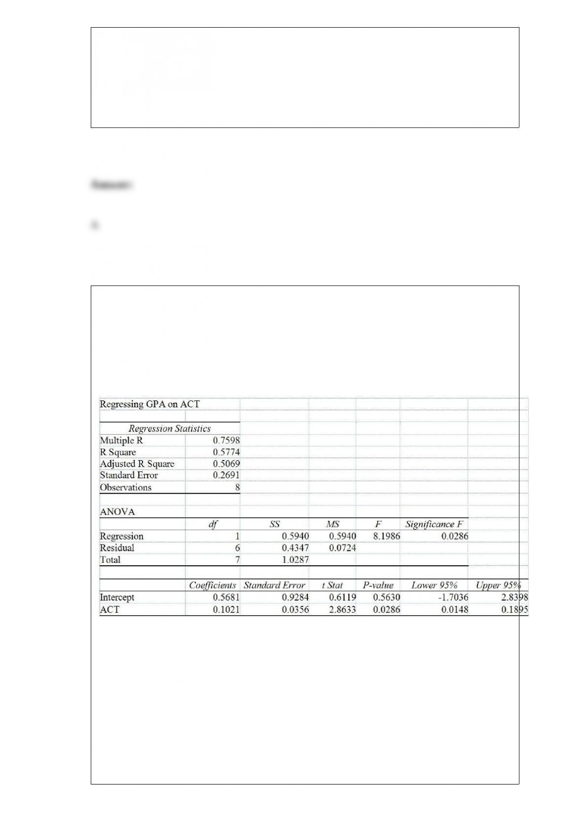
It is believed that GPA (grade point average, based on a four point scale) should have a
positive linear relationship with ACT scores. Given below is the Excel output for
predicting GPA using ACT scores based on a data set of 8 randomly chosen students
from a Big-Ten university.
Referring to Table 13-8, the interpretation of the coefficient of determination in this
regression is
A) 57.74% of the total variation of ACT scores can be explained by GPA.
B) ACT scores account for 57.74% of the total fluctuation in GPA.
C) GPA accounts for 57.74% of the variability of ACT scores.
D) None of the above.

The British Airways Internet site provides a questionnaire instrument that can be
answered electronically. Which of the 4 methods of data collection is involved when
people complete the questionnaire?
A) published sources
B) experimentation
C) surveying
D) observation
Referring to Table 14-17, which of the following is the correct null
hypothesis to determine whether there is a signiticant relationship
between the number of weeks a worker is unemployed due to a layof
and the entire set of explanatory variables?
TABLE 14-17
Given below are results from the regression analysis where the
dependent variable is the number of weeks a worker is unemployed
due to a layof (Unemploy) and the independent variables are the age
of the worker (Age) and a dummy variable for management position
(Manager: 1 = yes, 0 = no).
The results of the regression analysis are given below:

A) H0 : β0 = β1 = β2 = 0
B) H0 : β1 = β2 = 0
C) H0 : β0 = β1 = β2
D) H0 : β1 = β2
TABLE 17-8
The superintendent of a school district wanted to predict the percentage of students
passing a sixth-grade proficiency test. She obtained the data on percentage of students
passing the proficiency test (% Passing), daily mean of the percentage of students
attending class (% Attendance), mean teacher salary in dollars (Salaries), and
instructional spending per pupil in dollars (Spending) of 47 schools in the state.
Following is the multiple regression output with Y = % Passing as the dependent
variable, X1 = % Attendance, X2 = Salaries and X3 = Spending:
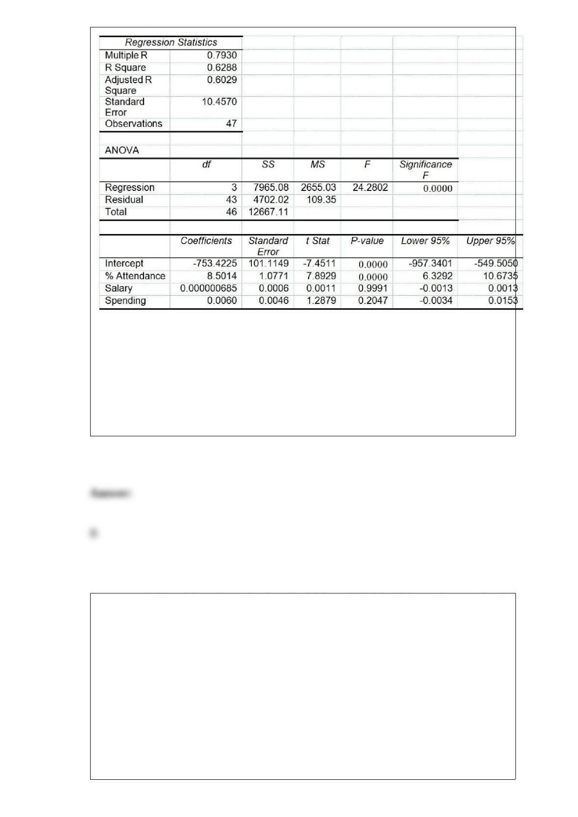
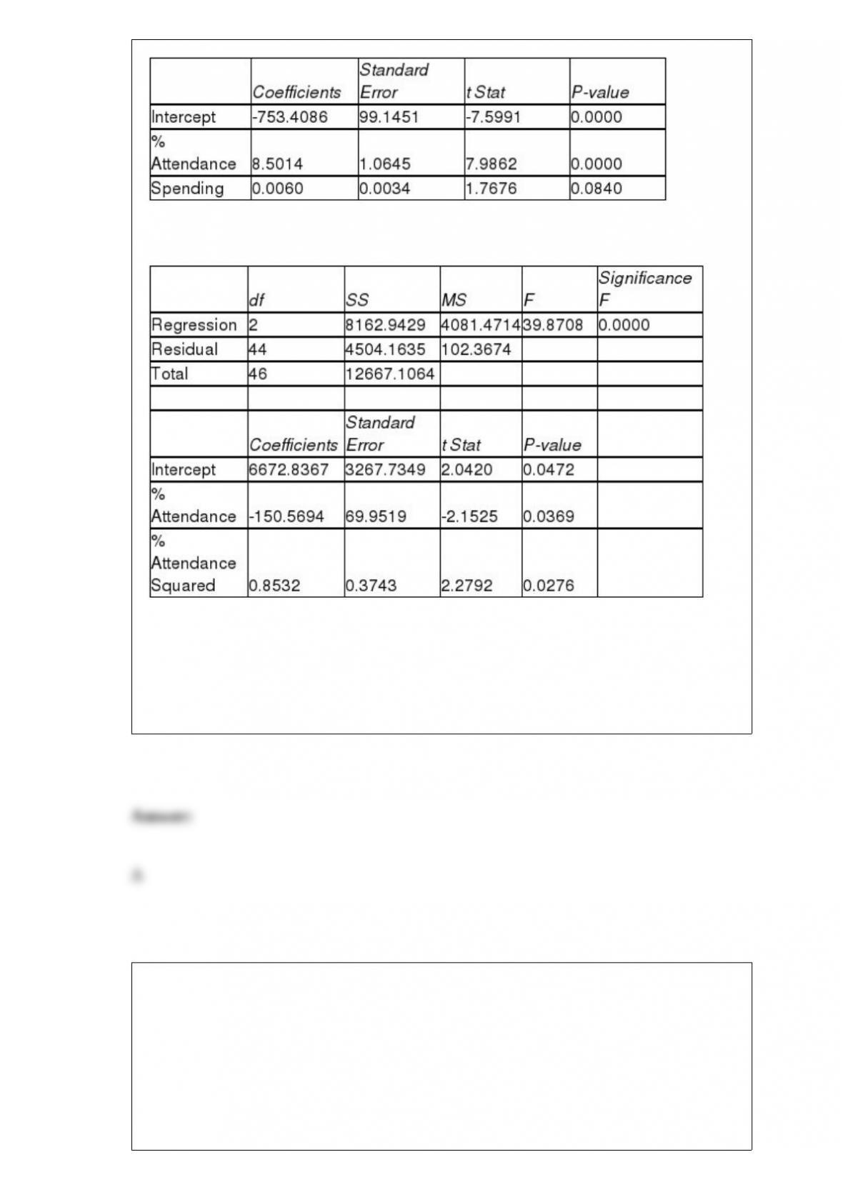
Referring to Table 17-8, which of the following is the correct null hypothesis to
determine whether there is a significant relationship between the percentage of students
passing the proficiency test and the entire set of explanatory variables?
A) H0 : β0 = β1 = β2 = β3 = 0
B) H0 : β1 = β2 = β3 = 0
C) H0 : β0 = β1 = β2 = β3 ≠0
D) H0 : β1 = β2 = β3 ≠0
An airline wants to select a computer software package for its reservation system. Four
software packages (1, 2, 3, and 4) are commercially available. The airline will choose
the package that bumps the fewest mean number of passengers as possible during a
month. An experiment is set up in which each package is used to make reservations for
5 randomly selected weeks. (A total of 20 weeks was included in the experiment.) The
number of passengers bumped each week is given below. How should the data be
analyzed?
Package 1: 12, 14, 9, 11, 16
Package 2: 2, 4, 7, 3, 1

Package 3: 10, 9, 6, 10, 12
Package 4: 7, 6, 6, 15, 12
A) F test for differences in variances
B) One-way ANOVA F test
C) t test for the differences in means
D) t test for the mean difference
TABLE 17-9
What are the factors that determine the acceleration time (in sec.) from 0 to 60 miles per
hour of a car? Data on the following variables for 171 different vehicle models were
collected:
Accel Time: Acceleration time in sec.
Cargo Vol: Cargo volume in cu. ft.
HP: Horsepower
MPG: Miles per gallon
SUV: 1 if the vehicle model is an SUV with Coupe as the base when SUV and Sedan
are both 0
Sedan: 1 if the vehicle model is a sedan with Coupe as the base when SUV and Sedan
are both 0
The regression results using acceleration time as the dependent variable and the
remaining variables as the independent variables are presented below.
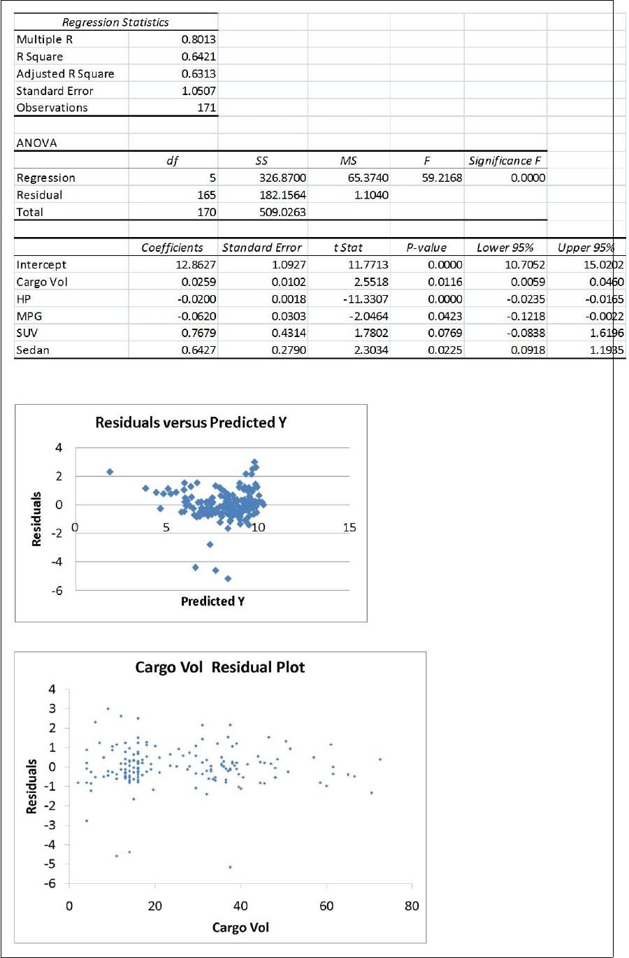
The various residual plots are as shown below.
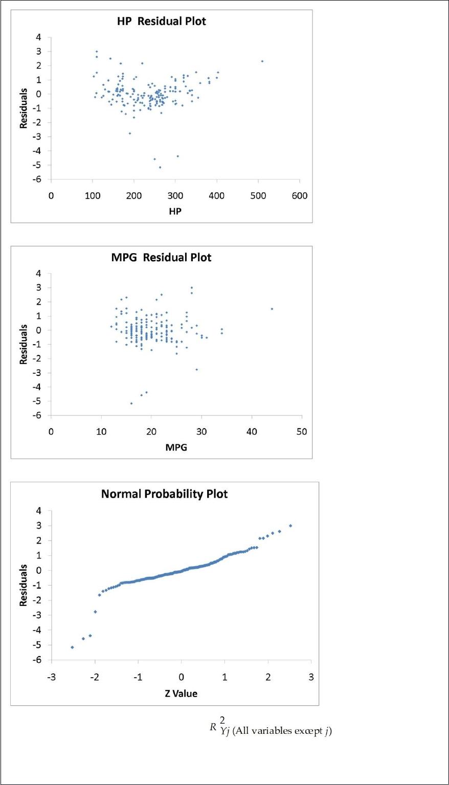
The coefficient of partial determination ( ) of each of the 5
predictors are, respectively, 0.0380, 0.4376, 0.0248, 0.0188, and 0.0312.
The coefficient of multiple determination for the regression model using each of the 5

variables Xj as the dependent variable and all other X variables as independent variables
( ) are, respectively, 0.7461, 0.5676, 0.6764, 0.8582, 0.6632.
Referring to Table 17-9, what is the correct interpretation for the estimated coefficient
for MPG?
A) As the miles per gallon decreases by one unit, the mean 0 to 60 miles per hour
acceleration time will increase by an estimated 0.0620 seconds without taking into
consideration all the other independent variables included in the model.
B) As the 0 to 60 miles per hour acceleration time decreases by one second, the mean
miles per gallon will increase by an estimated 0.0620 unit without taking into
consideration all the other independent variables included in the model.
C) As the miles per gallon decreases by one unit, the mean 0 to 60 miles per hour
acceleration time will increase by an estimated 0.0620 seconds taking into
consideration all the other independent variables included in the model.
D) As the 0 to 60 miles per hour acceleration time decreases by one second, the mean
miles per gallon will increase by an estimated 0.0620 unit taking into consideration all
the other independent variables included in the model.
If n = 10 and = 0.70, then the mean of the binomial distribution is
A) 0.07.
B) 1.45.
C) 7.00.
D) 14.29.
Referring to Table 14-6, what can we say about the regression model?
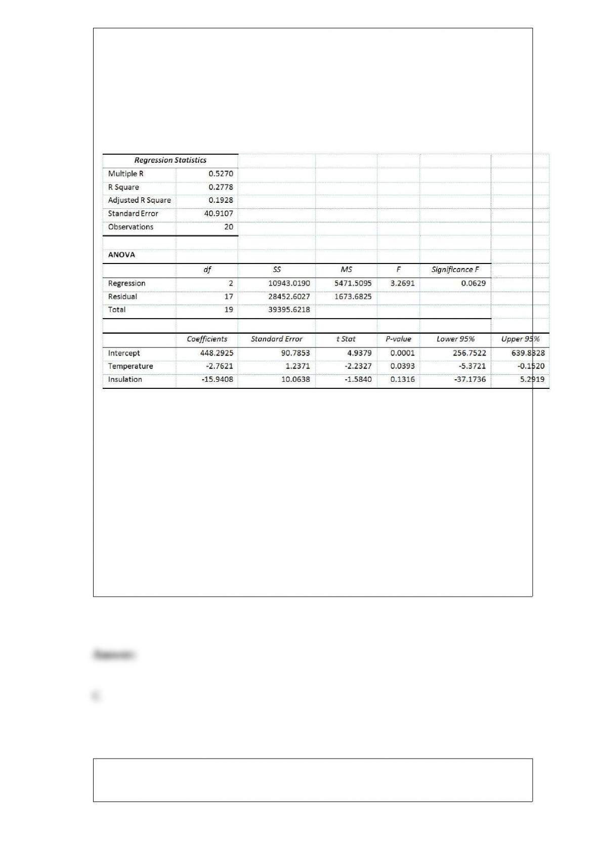
TABLE 14-6
One of the most common questions of prospective house buyers pertains to the cost of
heating in dollars (Y). To provide its customers with information on that matter, a large
real estate firm used the following 2 variables to predict heating costs: the daily
minimum outside temperature in degrees of Fahrenheit (X1) and the amount of
insulation in inches (X2). Given below is EXCEL output of the regression model.
Also SSR (X1∣ X2) = 8343.3572 and SSR (X2∣ X1) = 4199.2672
A) The model explains 17.12% of the variability of heating costs; after correcting for
the degrees of freedom, the model explains 27.78% of the sample variability of heating
costs.
B) The model explains 19.28% of the variability of heating costs; after correcting for
the degrees of freedom, the model explains 27.78% of the sample variability of heating
costs.
C) The model explains 27.78% of the variability of heating costs; after correcting for
the degrees of freedom, the model explains 19.28% of the sample variability of heating
costs.
D) The model explains 19.28% of the variability of heating costs; after correcting for
the degrees of freedom, the model explains 17.12% of the sample variability of heating
costs.
TABLE 15-4
The superintendent of a school district wanted to predict the percentage of students
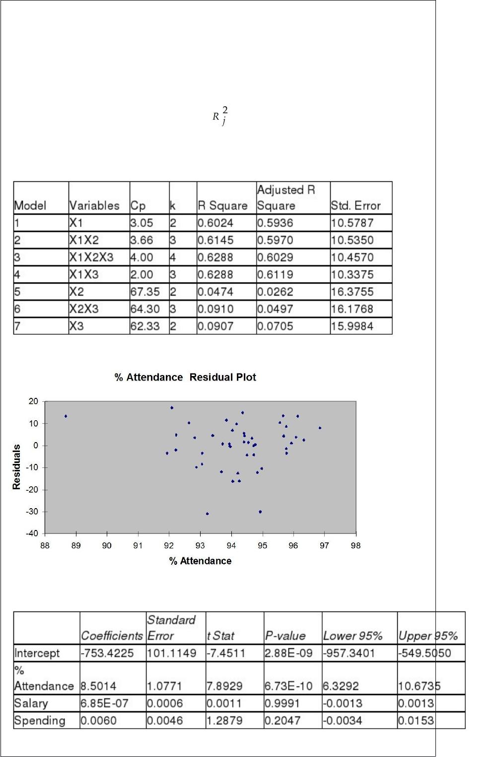
passing a sixth-grade proficiency test. She obtained the data on percentage of students
passing the proficiency test (% Passing), daily mean of the percentage of students
attending class (% Attendance), mean teacher salary in dollars (Salaries), and
instructional spending per pupil in dollars (Spending) of 47 schools in the state.
Let Y = % Passing as the dependent variable, X1 = % Attendance, X2 = Salaries and X3
= Spending.
The coefficient of multiple determination ( ) of each of the 3 predictors with all the
other remaining predictors are, respectively, 0.0338, 0.4669, and 0.4743.
The output from the best-subset regressions is given below:
Following is the residual plot for % Attendance:
Following is the output of several multiple regression models:
Model (I):
Model (II):
Model (III):
Referring to Table 15-4, the “best” model chosen using the adjusted R-square statistic is
A) X1, X3.
B) X1, X2, X3.
C) Either of the above
D) None of the above
For some value of Z, the value of the cumulative standardized normal distribution is
0.2090. The value of Z is
A) -0.81.
B) -0.31.
C) 0.31.
D) 1.96.
TABLE 17-6
A weight-loss clinic wants to use regression analysis to build a model for weight loss of
a client (measured in pounds). Two variables thought to affect weight loss are client’s
length of time on the weight-loss program and time of session. These variables are
described below:
Y = Weight loss (in pounds)
X1 = Length of time in weight-loss program (in months)
X2 = 1 if morning session, 0 if not
X3 = 1 if afternoon session, 0 if not (Base level = evening session)
Data for 12 clients on a weight-loss program at the clinic were collected and used to fit
the interaction model:
Y = β0 + β1X1 + β2X2 + β3X3 + β4X1X2 + β5X1X3 + ε
Partial output from Microsoft Excel follows:
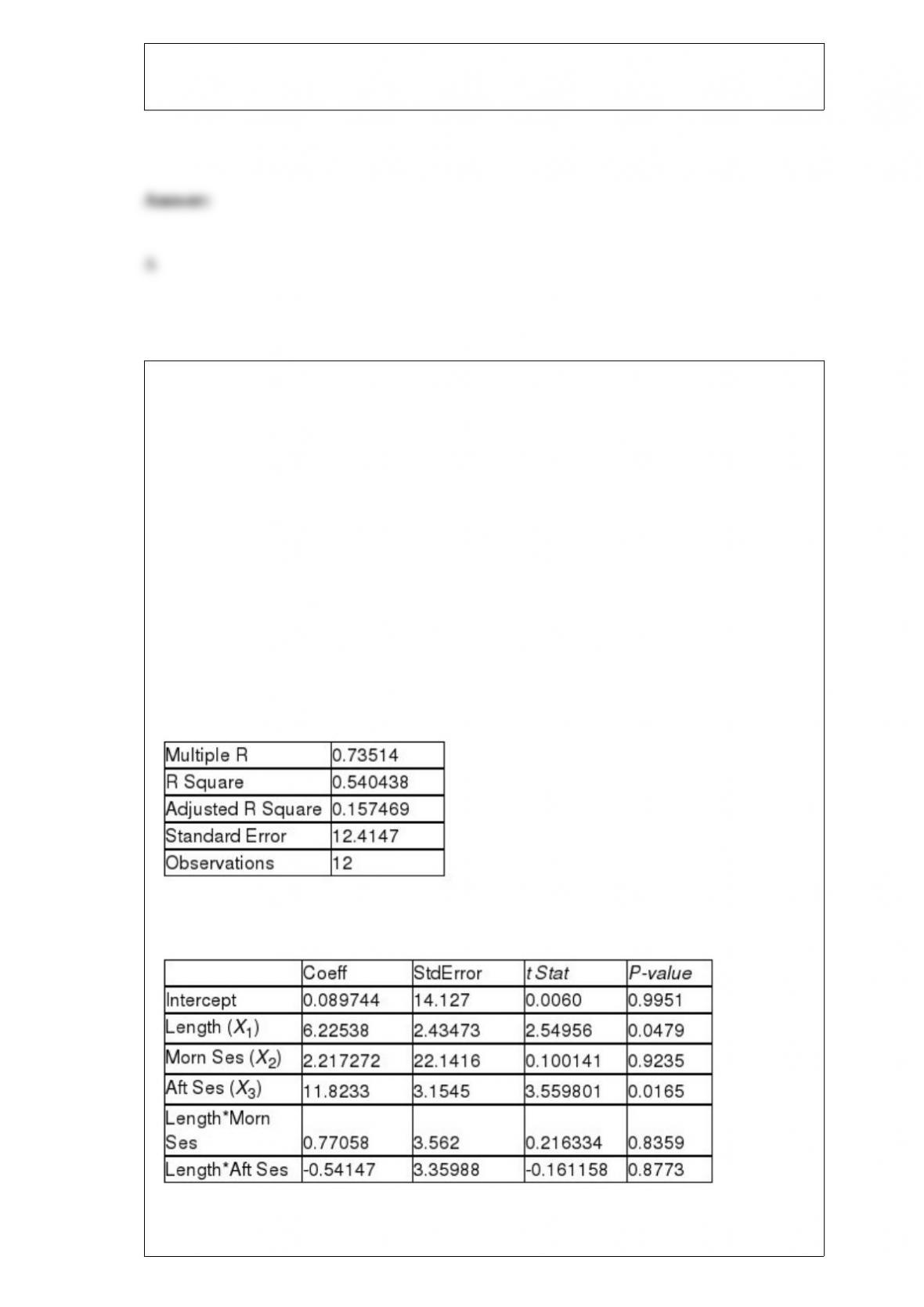
Regression Statistics
ANOVA
F = 5.41118 Significance F = 0.040201
Referring to Table 17-6, what null hypothesis would you test to determine whether the
slope of the linear relationship between weight loss (Y) and time in the program (X1)
varies according to time of session?
A) H0 : β1 = β2 = β3 = β4 = β5 = 0
B) H0 : β2 = β3 = β4 = β5 = 0
C) H0 : β4 = β5 = 0
D) H0 : β2 = β3 = 0
TABLE 11-7
A campus researcher wanted to investigate the factors that affect visitor travel time in a
complex, multilevel building on campus. Specifically, he wanted to determine whether
different building signs (building maps versus wall signage) affect the total amount of
time visitors require to reach their destination and whether that time depends on
whether the starting location is inside or outside the building. Three subjects were
assigned to each of the combinations of signs and starting locations, and travel time in
seconds from beginning to destination was recorded. An Excel output of the appropriate
analysis is given below:
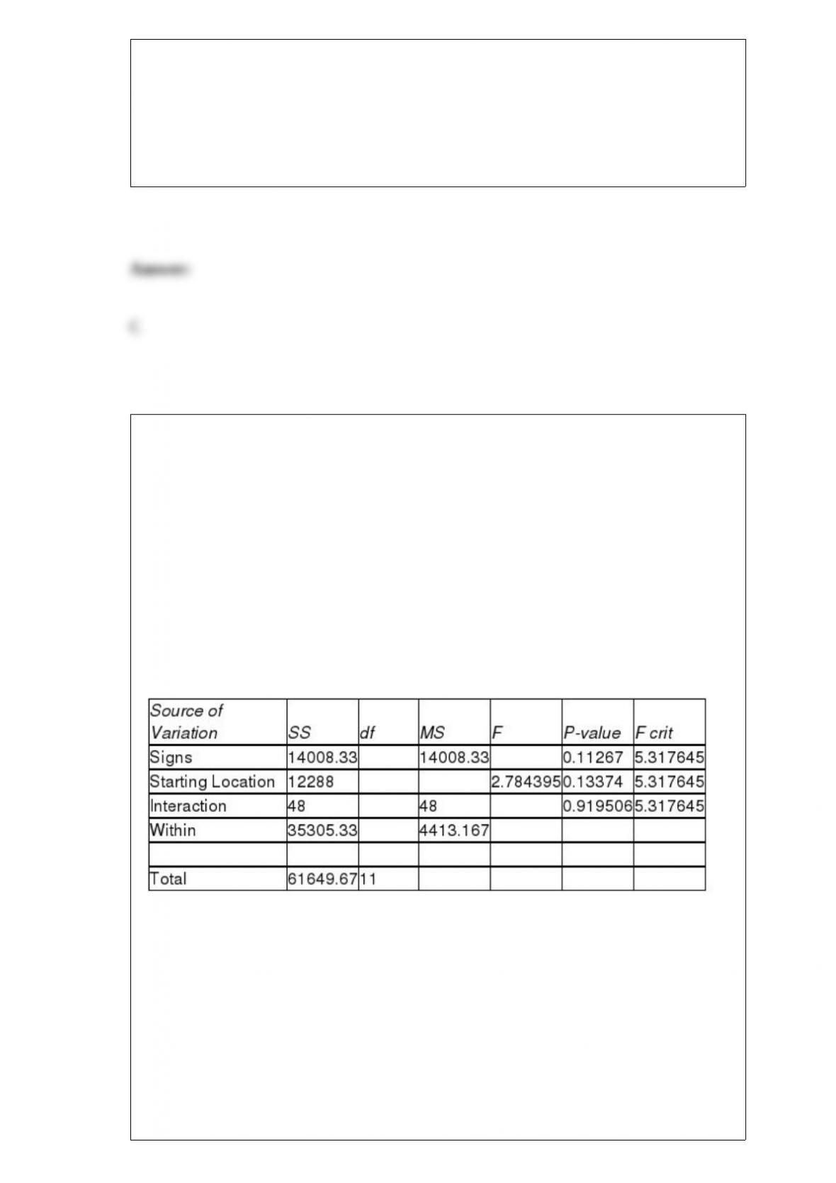
ANOVA
Referring to Table 11-7, the F test statistic for testing the interaction effect between the
types of signs and the starting location is
A) 0.0109.
B) 2.7844.
C) 3.1742.
D) 5.3176.
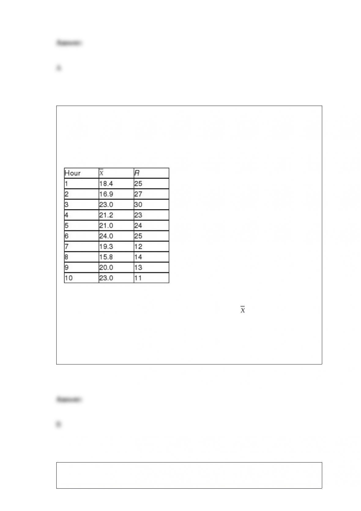
TABLE 18-4
A factory supervisor is concerned that the time it takes workers to complete an
important production task (measured in seconds) is too erratic and adversely affects
expected profits. The supervisor proceeds by randomly sampling 5 individuals per hour
for a period of 10 hours. The sample mean and range for each hour are listed below.
She also decides that lower and upper specification limit for the critical-to-quality
variable should be 10 and 30 seconds, respectively.
Referring to Table 18-4, suppose the supervisor constructs an chart to see if the
process is in-control. Which expression best describes this chart?
A) Decreasing trend
B) In-control
C) Increasing trend
D) Individual outliers
A professor receives, on average, 24.7 e-mails from students the day before the midterm
exam. To compute the probability of receiving at least 10 e-mails on such a day, he will

use what type of probability distribution?
A) Binomial distribution
B) Poisson distribution
C) Hypergeometric distribution
D) None of the above.
The owner of a local nightclub has recently surveyed a random sample of n = 250
customers of the club. She would now like to determine whether or not the mean age of
her customers is greater than 30. If so, she plans to alter the entertainment to appeal to
an older crowd. If not, no entertainment changes will be made. Suppose she found that
the sample mean was 30.45 years and the sample standard deviation was 5 years. If she
wants to have a level of significance at 0.01, what decision should she make?
A) Reject H0.
B) Reject H1.
C) Do not reject H0.
D) We cannot tell what her decision should be from the information given.
TABLE 11-7
A campus researcher wanted to investigate the factors that affect visitor travel time in a
complex, multilevel building on campus. Specifically, he wanted to determine whether

different building signs (building maps versus wall signage) affect the total amount of
time visitors require to reach their destination and whether that time depends on
whether the starting location is inside or outside the building. Three subjects were
assigned to each of the combinations of signs and starting locations, and travel time in
seconds from beginning to destination was recorded. An Excel output of the appropriate
analysis is given below:
ANOVA
Referring to Table 11-7, the mean squares for starting location (factor B) is
A) 48.
B) 4,413.17.
C) 12,288.
D) 14,008.3.
TABLE 13-7
An investment specialist claims that if one holds a portfolio that moves in the opposite
direction to the market index like the S&P 500, then it is possible to reduce the
variability of the portfolio’s return. In other words, one can create a portfolio with
positive returns but less exposure to risk.
A sample of 26 years of S&P 500 index and a portfolio consisting of stocks of private
prisons, which are believed to be negatively related to the S&P 500 index, is collected.
A regression analysis was performed by regressing the returns of the prison stocks
portfolio (Y) on the returns of S&P 500 index (X) to prove that the prison stocks

portfolio is negatively related to the S&P 500 index at a 5% level of significance. The
results are given in the following EXCEL output.
Referring to Table 13-7, which of the following will be a correct conclusion?
A) You cannot reject the null hypothesis and, therefore, conclude that there is sufficient
evidence to show that the prisons stock portfolio and S&P 500 index are negatively
related.
B) You can reject the null hypothesis and, therefore, conclude that there is sufficient
evidence to show that the prisons stock portfolio and S&P 500 index are negatively
related.
C) You cannot reject the null hypothesis and, therefore, conclude that there is
insufficient evidence to show that the prisons stock portfolio and S&P 500 index are
negatively related.
D) You can reject the null hypothesis and conclude that there is insufficient evidence to
show that the prisons stock portfolio and S&P 500 index are negatively related.
TABLE 17-1
A real estate builder wishes to determine how house size (House) is influenced by
family income (Income), family size (Size), and education of the head of household
(School). House size is measured in hundreds of square feet, income is measured in
thousands of dollars, and education is in years. The builder randomly selected 50
families and ran the multiple regression. Microsoft Excel output is provided below:
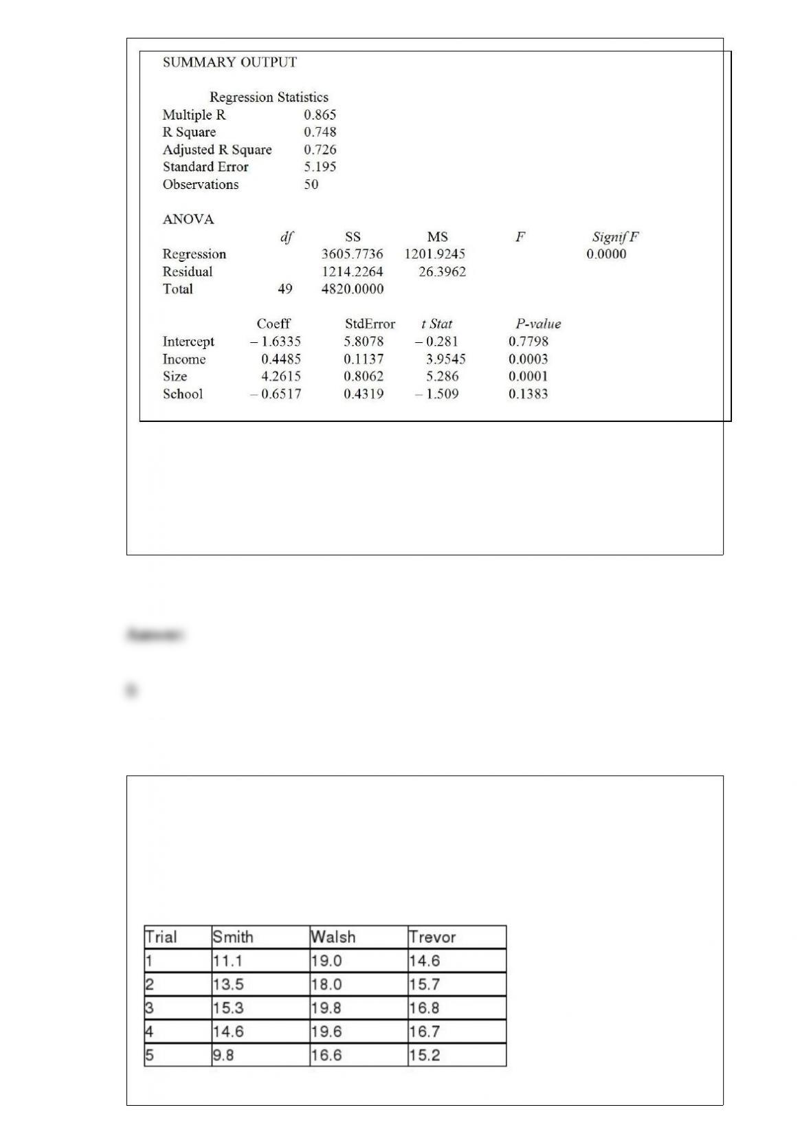
Referring to Table 17-1, which of the independent variables in the model are significant
at the 5% level?
A) Income, Size, School
B) Income, Size
C) Size, School
D) Income, School
TABLE 11-4
An agronomist wants to compare the crop yield of 3 varieties of chickpea seeds. She
plants 15 fields, 5 with each variety. She then measures the crop yield in bushels per
acre. Treating this as a completely randomized design, the results are presented in the
table that follows.

Referring to Table 11-4, state the null hypothesis that can be tested.
TABLE 8-13
A wealthy real estate investor wants to decide whether it is a good investment to build a
high-end shopping complex in a suburban county in Houston. His main concern is the
total market value of the 3,605 houses in the suburban county. He commissioned a
statistical consulting group to take a sample of 200 houses and obtained a sample mean
market price of $225,000 and a sample standard deviation of $38,700. The consulting
group also found out that the mean differences between market prices and appraised
prices was $125,000 with a standard deviation of $3,400. Also the proportion of houses
in the sample that are appraised for higher than the market prices is 0.24.
Referring to Table 8-13, if he wants a 95% confidence on estimating the true population
mean market price of the houses in the suburban county to be within $10,000, how
large a sample will he need?
TABLE 3-1
Health care issues are receiving much attention in both academic and political arenas. A
sociologist recently conducted a survey of citizens over 60 years of age whose net
worth is too high to qualify for Medicaid. The ages of 25 senior citizens were as
follows:
Referring to Table 3-1, determine the median age of the senior citizens.
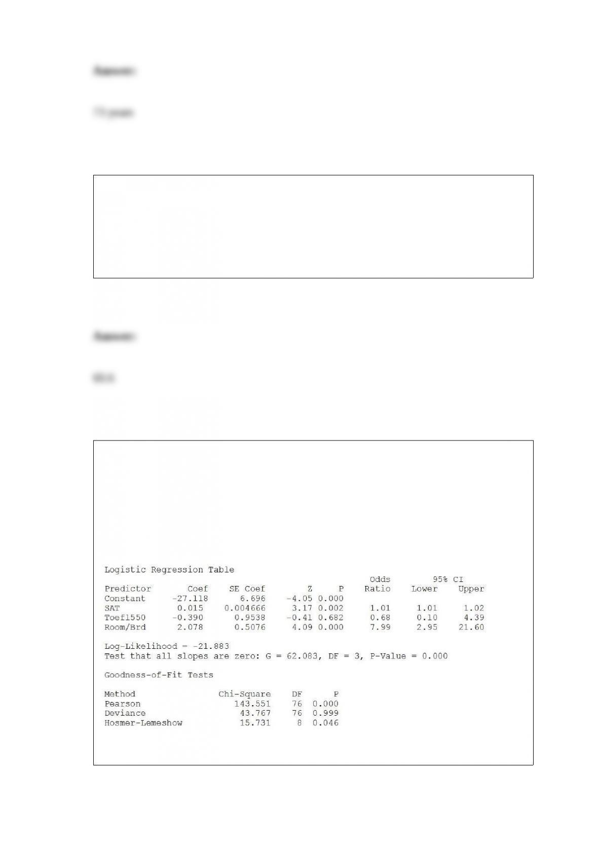
TABLE 16-5
The number of passengers arriving at San Francisco on the Amtrak cross-country
express on 6 successive Mondays were: 60, 72, 96, 84, 36, and 48.
Referring to Table 16-5, the number of arrivals will be exponentially smoothed with a
smoothing constant of 0.25. The forecast of the number of arrivals on the seventh
Monday will be ________.
TABLE 17-11
A logistic regression model was estimated in order to predict the probability that a
randomly chosen university or college would be a private university using information
on mean total Scholastic Aptitude Test score (SAT) at the university or college, the
room and board expense measured in thousands of dollars (Room/Brd), and whether the
TOEFL criterion is at least 550 (Toefl550 = 1 if yes, 0 otherwise.) The dependent
variable, Y, is school type (Type = 1 if private and 0 otherwise).
Referring to Table 17-11, what are the degrees of freedom for the chi-square
distribution when testing whether the model is a good-fitting model?

TABLE 6-1
The number of column inches of classified advertisements appearing on Mondays in a
certain daily newspaper is normally distributed with a population mean of 320 and a
population standard deviation of 20 inches.
Referring to Table 6-1, for a randomly chosen Monday, what is the probability that
there will be less than 340 column inches of classified advertisement?
TABLE 3-2
The data below represent the amount of grams of carbohydrates in a serving of
breakfast cereal in a sample of 11 different servings.
Referring to Table 3-2, is the carbohydrate amount in the cereal right- or left-skewed?
TABLE 17-11
A logistic regression model was estimated in order to predict the probability that a
randomly chosen university or college would be a private university using information
on mean total Scholastic Aptitude Test score (SAT) at the university or college, the
room and board expense measured in thousands of dollars (Room/Brd), and whether the

TOEFL criterion is at least 550 (Toefl550 = 1 if yes, 0 otherwise.) The dependent
variable, Y, is school type (Type = 1 if private and 0 otherwise).
Referring to Table 17-11, what is the p-value of the test statistic when testing whether
SAT makes a significant contribution to the model in the presence of the other
independent variables?