TABLE 14-16
What are the factors that determine the acceleration time (in sec.)
from 0 to 60 miles per hour of a car? Data on the following variables
for 30 different vehicle models were collected:
Y (Accel Time): Acceleration time in sec.
X1 (Engine Size): c.c.
X2 (Sedan): 1 if the vehicle model is a sedan and 0 otherwise
The regression results using acceleration time as the dependent
variable and the remaining variables as the independent variables are
presented below.
The various residual plots are as shown below.

The coe,cient of partial determinations and are 0.3301,
and 0.0594, respectively.
The coe,cient of determination for the regression model using each
of the 2 independent variables as the dependent variable and the
other independent variable as independent variables ( ) are,
respectively 0.0077, and 0.0077.
True or False: Referring to Table 14-16, the errors (residuals) appear to
be right-skewed.
TABLE 12-7
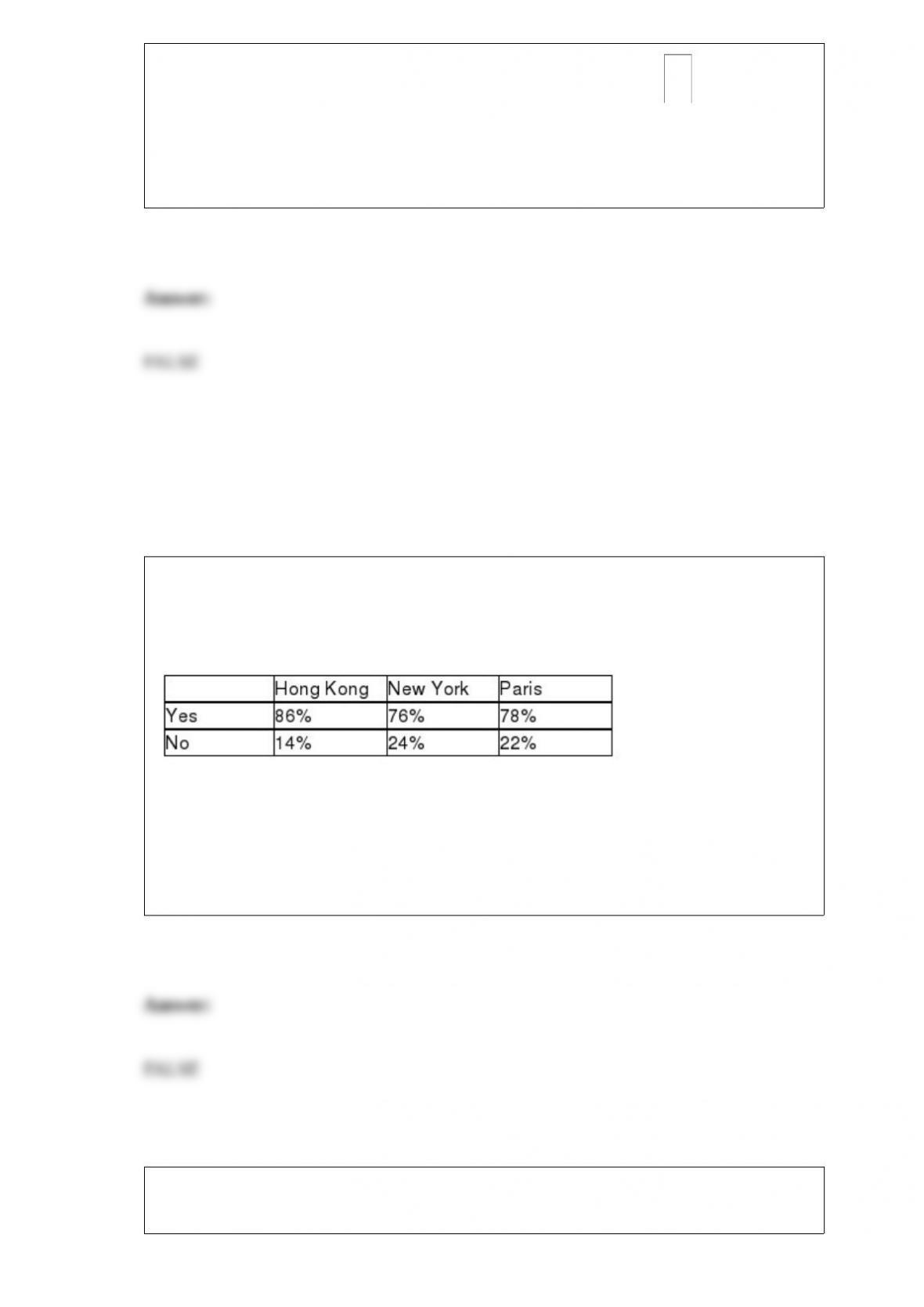
Data on the percentage of 200 hotels in each of the three large cities across the world on
whether minibar charges are correctly posted at checkout are given below.
At the 0.05 level of significance, you want to know if there is evidence of a difference
in the proportion of hotels that correctly post minibar charges among the three cities.
True or False: Referring to Table 12-7, the decision made suggests that the 3 cities all
have different proportions of hotels that correctly post minibar charges.
True or False: The difference between the lower limit of a confidence interval and the
point estimate used in constructing the confidence interval is called the sampling error.
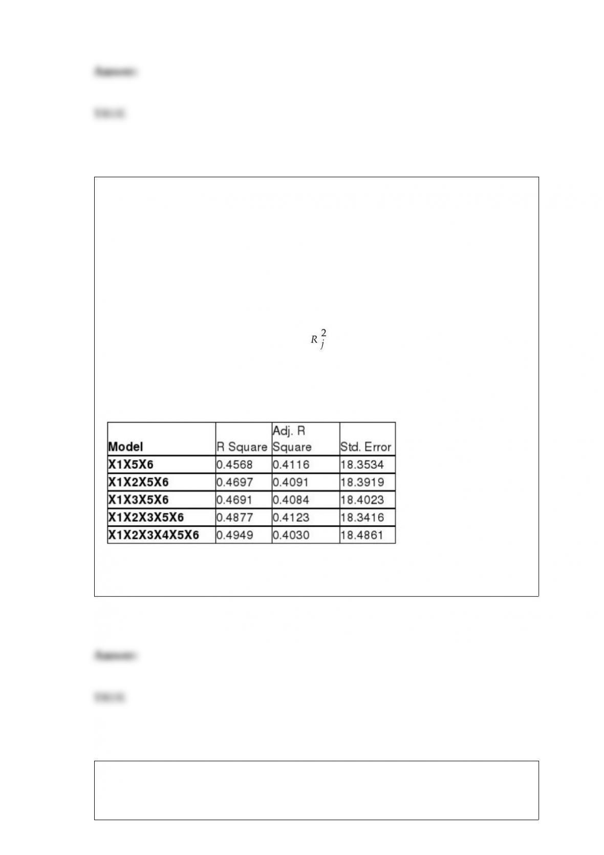
TABLE 15-6
Given below are results from the regression analysis on 40 observations where the
dependent variable is the number of weeks a worker is unemployed due to a layoff (Y)
and the independent variables are the age of the worker (X1), the number of years of
education received (X2), the number of years at the previous job (X3), a dummy variable
for marital status (X4: 1 = married, 0 = otherwise), a dummy variable for head of
household (X5: 1 = yes, 0 = no) and a dummy variable for management position (X6: 1
= yes, 0 = no).
The coefficient of multiple determination ( ) for the regression model using each of
the 6 variables Xj as the dependent variable and all other X variables as independent
variables are, respectively, 0.2628, 0.1240, 0.2404, 0.3510, 0.3342 and 0.0993.
The partial results from best-subset regression are given below:
True or False: Referring to Table 15-6, the model that includes X1, X3, X5 and X6 should
be among the appropriate models using the Mallow’s Cp statistic.
TABLE 11-3
As part of an evaluation program, a sporting goods retailer wanted to compare the
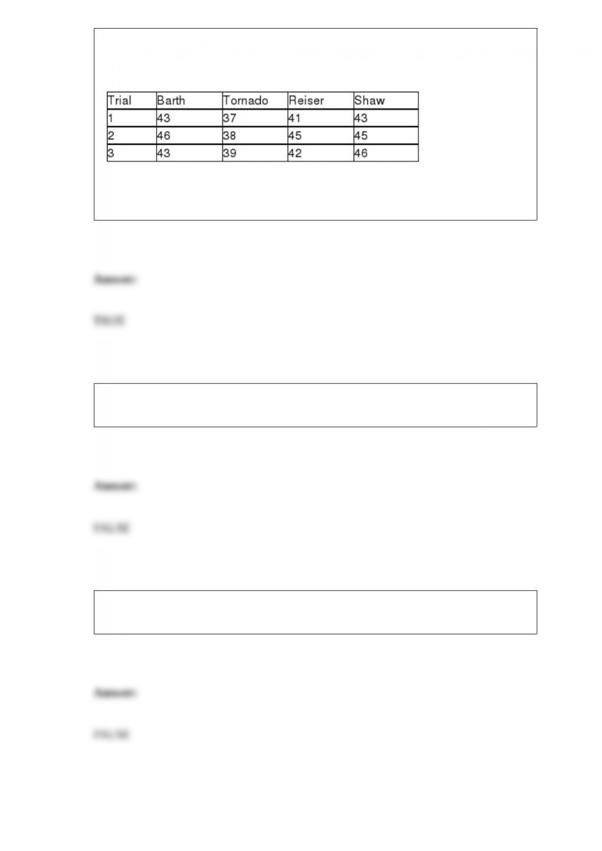
downhill coasting speeds of 4 brands of bicycles. She took 3 of each brand and
determined their maximum downhill speeds. The results are presented in miles per hour
in the table below.
True or False: Referring to Table 11-3, the test is valid only if the population of speeds
is normally distributed.
True or False: A process capability is estimated by the percentage of product or service
that fall outside the specification limits.
True or False: The question “Is your household income last year somewhere between
$50,000 and $100,000?” will most likely result in coverage error.
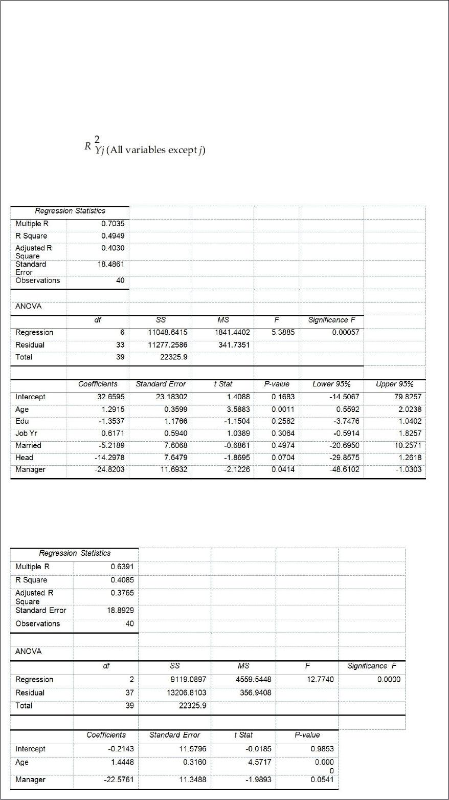
True or False: TABLE 17-10
Given below are results from the regression analysis where the dependent variable is
the number of weeks a worker is unemployed due to a layoff (Unemploy) and the
independent variables are the age of the worker (Age), the number of years of education
received (Edu), the number of years at the previous job (Job Yr), a dummy variable for
marital status (Married: 1 = married, 0 = otherwise), a dummy variable for head of
household (Head: 1 = yes, 0 = no) and a dummy variable for management position
(Manager: 1 = yes, 0 = no). We shall call this Model 1. The coefficient of partial
determination ( ) of each of the 6 predictors are, respectively,
0.2807, 0.0386, 0.0317, 0.0141, 0.0958, and 0.1201.
Model 2 is the regression analysis where the dependent variable is Unemploy and the
independent variables are Age and Manager. The results of the regression analysis are
given below:
Referring to Table 17-10, Model 1, we can conclude that, holding constant the effect of
the other independent variables, the number of years of education received has no
impact on the mean number of weeks a worker is unemployed due to a layoff at a 1%
level of significance if all we have is the information of the 95% confidence interval
estimate forβ2.
True or False: When using the X2 tests for independence, you should be aware that
expected frequencies that are too small will lead to a large Type I error.
True or False: As a population becomes large, it is usually better to obtain statistical
information from the entire population.

TABLE 8-10
A sales and marketing management magazine conducted a survey on salespeople
cheating on their expense reports and other unethical conduct. In the survey on 200
managers, 58% of the managers have caught salespeople cheating on an expense report,
50% have caught salespeople working a second job on company time, 22% have caught
salespeople listing a ‘strip bar” as a restaurant on an expense report, and 19% have
caught salespeople giving a kickback to a customer.
True or False: Referring to Table 8-10, we are 95% confident that the population mean
number of managers who have caught salespeople cheating on an expense report is
between 0.5116 to 0.6484.
Referring to Table 14-13, the 5tted model for predicting demand in
San Francisco is ________.
TABLE 14-13
An econometrician is interested in evaluating the relationship of
demand for building materials to mortgage rates in Los Angeles and
San Francisco. He believes that the appropriate model is
Y = 10 + 5X1 + 8X2
where X1 = mortgage rate in %
X2 = 1 if SF, 0 if LA
Y = demand in $100 per capita
A) 10 + 5X1
B) 10 + 13X1
C) 15 + 8X2
D) 18 + 5X1

TABLE 9-2
A student claims that he can correctly identify whether a person is a business major or
an agriculture major by the way the person dresses. Suppose in actuality that if someone
is a business major, he can correctly identify that person as a business major 87% of the
time. When a person is an agriculture major, the student will incorrectly identify that
person as a business major 16% of the time. Presented with one person and asked to
identify the major of this person (who is either a business or an agriculture major), he
considers this to be a hypothesis test with the null hypothesis being that the person is a
business major and the alternative that the person is an agriculture major.
Referring to Table 9-2, what is the value of ?
A) 0.13
B) 0.16
C) 0.84
D) 0.87
Which of the following is not part of the DMAIC process in Six Sigma management?
A) Define
B) Do
C) Analyze
D) Control
The director of a training program wanted to know if a one-week orientation would
change the perception of potential clients who would perceive the program as being
good. He collected information on the number of clients who would rate the program as
being good before and after the orientation. Which of the following tests will be the
most appropriate?
A) χ2 test for proportions
B) McNemar test
C) Wilcoxon rank sum test
D) Tukey-Kramer procedure
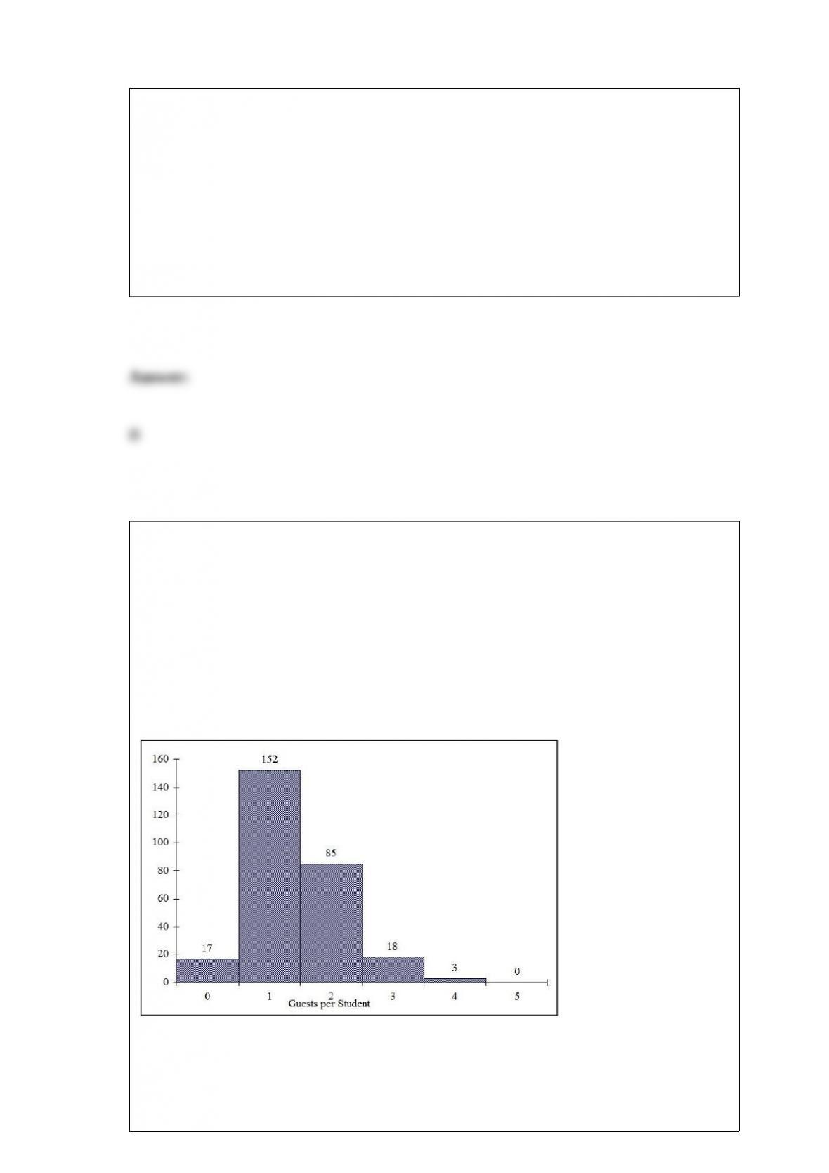
TABLE 2-3
Every spring semester, the School of Business coordinates a luncheon with local
business leaders for graduating seniors, their families, and friends. Corporate
sponsorship pays for the lunches of each of the seniors, but students have to purchase
tickets to cover the cost of lunches served to guests they bring with them. The following
histogram represents the attendance at the senior luncheon, where X is the number of
guests each graduating senior invited to the luncheon and f is the number of graduating
seniors in each category.
Referring to the histogram from Table 2-3, if all the tickets purchased were used, how
many guests attended the luncheon?
A) 4
B) 152
C) 275
D) 388
You have created a 95% confidence interval for μ with the result 10 15. What
decision will you make if we test H0 : = 16 versus H1 : ≠16 at = 0.01?
A) Reject H0 in favor of H1.
B) Do not reject H0 in favor of H1.
C) Fail to reject H0 in favor of H1.
D) You cannot tell what our decision will be from the information given.
In a local cellular phone area, company A accounts for 60% of the cellular phone

market, while company B accounts for the remaining 40% of the market. Of the cellular
calls made with company A, 1% of the calls will have some sort of interference, while
2% of the cellular calls with company B will have interference. If a cellular call is
selected at random and has interference, what is the probability that it was with
company A?
A) 0.071
B) 0.429
C) 0.571
D) It cannot be determined.
An airline wants to select a computer software package for its reservation system. Four
software packages (1, 2, 3, and 4) are commercially available. An experiment is set up
in which each package is used to make reservations for 5 randomly selected weeks and
data on the number of passengers that are bumped over a month are collected. (A total
of 20 weeks was included in the experiment.) The variance on the number of passengers
that are bumped is found to be roughly the same for the 4 packages. Which of the
following tests will be the most appropriate to find out if the mean number of
passengers being bumped over a month is the same across the 4 packages?
A) Paired t test
B) Pooled-variance t test
C) One-way ANOVA F test for differences among more than two means
D) Two-way ANOVA F test for interaction effect
Referring to Table 14-3, one economy in the sample had an aggregate consumption
level of $4 billion, a GDP of $6 billion, and an aggregate price level of 200. What is the
residual for this data point?
TABLE 14-3
An economist is interested to see how consumption for an economy (in $ billions) is
influenced by gross domestic product ($ billions) and aggregate price (consumer price
index). The Microsoft Excel output of this regression is partially reproduced below.
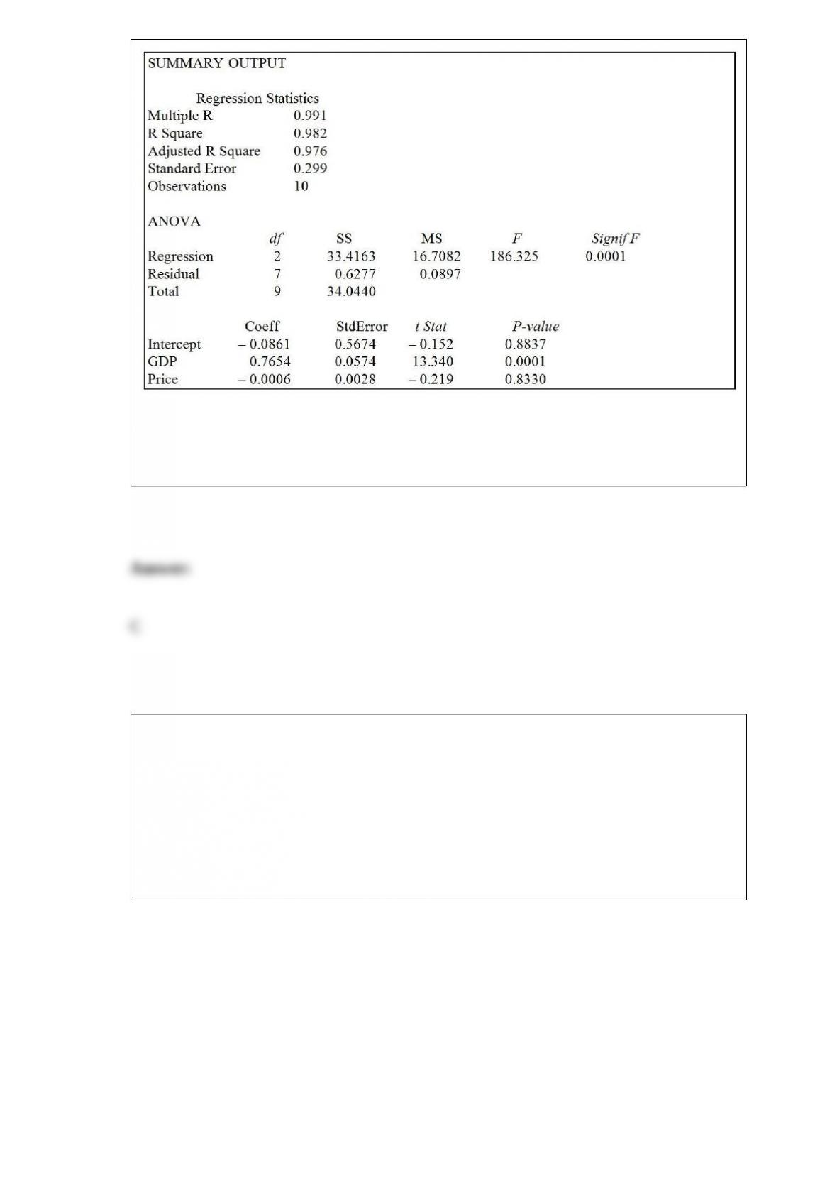
A) $4.39 billion
B) $0.39 billion
C) -$0.39 billion
D) -$1.33 billion
Referring to Table 14-4, what are the residual degrees of freedom that are missing from
the output?
TABLE 14-4
A real estate builder wishes to determine how house size (House) is influenced by
family income (Income) and family size (Size). House size is measured in hundreds of
square feet and income is measured in thousands of dollars. The builder randomly
selected 50 families and ran the multiple regression. Partial Microsoft Excel output is
provided below:
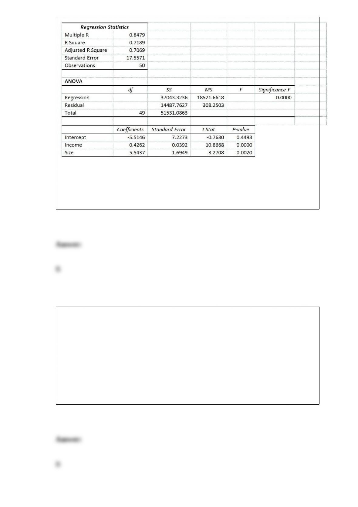
Also SSR (X1∣ X2) = 36400.6326 and SSR (X2∣ X1) = 3297.7917
A) 2
B) 47
C) 49
D) 50
A buyer for a manufacturing plant suspects that his primary supplier of raw materials is
overcharging. In order to determine if his suspicion is correct, he contacts a second
supplier and asks for the prices on various identical materials. He wants to compare
these prices with those of his primary supplier. He collected data on 6 different
materials from both suppliers. He believes that the differences are normally distributed.
Which of the following tests will be the most appropriate?
A) Pooled-variance t test
B) Paired t test
C) Wilcoxon rank sum test
D) McNemar test

Which of the following best measures the ability of a process to consistently meet
specified customer-driven requirements?
A) Process capability
B) Specification limits
C) Upper control limit
D) Lower control limit
TABLE 1-2
A Wall Street Journal poll asked 2,150 adults in the United States a series of questions
to find out their view on the U.S. economy.
Referring to Table 1-2, the possible responses to the question “Are you 1. Currently
employed,
2. Unemployed but actively looking for job, 3. Unemployed and quit looking for job?”
result in
A) a nominal scale variable.
B) an ordinal scale variable.
C) an interval scale variable.
D) a ratio scale variable.
Which of the following sampling methods is a probability sample?
A) convenience sample

B) quota sample
C) stratified sample
D) judgment sample
A university system enrolling hundreds of thousands of students is considering a change
in the way students pay for their education. Currently, the students pay $400 per credit
hour. The university system administrators are contemplating charging each student a
set fee of $7,000 per quarter, regardless of how many credit hours each takes. To see if
this proposal would be economically feasible, the administrators would like to know
how many credit hours, on the average, each student takes per quarter. A random
sample of 250 students yields a mean of 14.1 credit hours per quarter and a standard
deviation of 2.3 credit hours per quarter. Suppose the administration wanted to estimate
the mean to within 0.1 hours at 95% reliability and assumed that the sample standard
deviation provided a good estimate for the population standard deviation. How large a
total sample would they need to take?
TABLE 4-8
According to the record of the registrar’s office at a state university, 35% of the students
are freshman, 25% are sophomore, 16% are junior and the rest are senior. Among the
freshmen, sophomores, juniors and seniors, the portion of students who live in the
dormitory are, respectively, 80%, 60%, 30% and 20%.
Referring to Table 4-8, what is the probability that a randomly selected student is a
sophomore who does not live in a dormitory?
The true length of boards cut at a mill with a listed length of 10 feet is normally
distributed with a mean of 123 inches and a standard deviation of 1 inch. What
proportion of the boards will be between 121 and 124 inches?
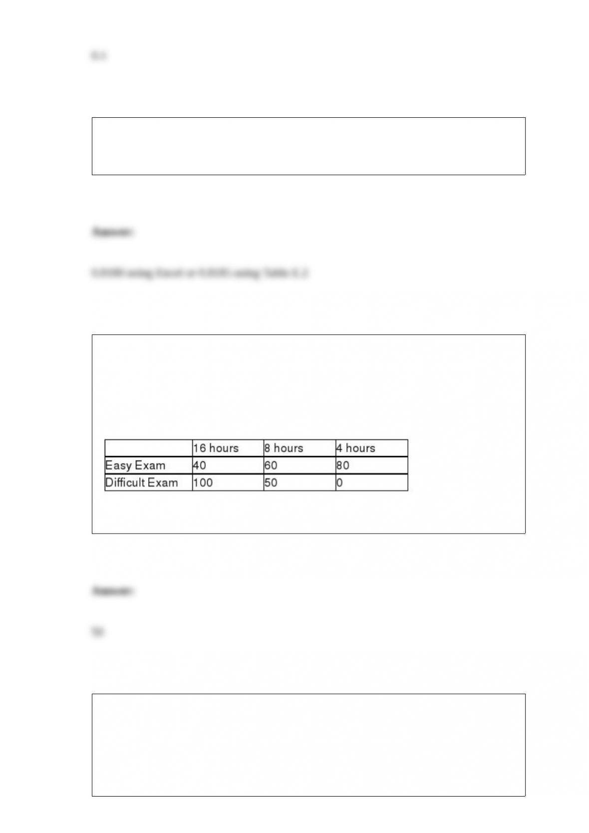
TABLE 19-6
A student wanted to find out the optimal strategy to study for a Business Statistics
exam. He constructed the following payoff table based on the mean amount of time he
needed to study every week for the course and the degree of difficulty of the exam.
From the information that he gathered from students who had taken the course, he
concluded that there was a 40% probability that the exam would be easy.
Referring to Table 19-6, what is the opportunity loss of spending 8 hours per week on
average studying for the exam when the exam turns out to be difficult?
Referring to Table 14-16, ________ of the variation in Accel Time can be
explained by the two independent variables.
TABLE 14-16
What are the factors that determine the acceleration time (in sec.)

from 0 to 60 miles per hour of a car? Data on the following variables
for 30 different vehicle models were collected:
Y (Accel Time): Acceleration time in sec.
X1 (Engine Size): c.c.
X2 (Sedan): 1 if the vehicle model is a sedan and 0 otherwise
The regression results using acceleration time as the dependent
variable and the remaining variables as the independent variables are
presented below.
The various residual plots are as shown below.

The coe,cient of partial determinations and are 0.3301,
and 0.0594, respectively.
The coe,cient of determination for the regression model using each
of the 2 independent variables as the dependent variable and the

other independent variable as independent variables ( ) are,
respectively 0.0077, and 0.0077.