True or False: The procedure for the Wilcoxon rank sum test requires that you rank each
group separately rather than together.
True or False: The method of least squares may be used to estimate both linear and
curvilinear trends.
True or False: A high value of R2 significantly above 0 in multiple regression
accompanied by insignificant t-values on all parameter estimates very often indicates a
high correlation between independent variables in the model.
TABLE 8-12
A random sample of 100 stores from a large chain of 500 garden supply stores was
selected to determine the mean number of lawnmowers sold at an end-of-season
clearance sale. The sample results indicated a mean of 6 and a standard deviation of 2
lawnmowers sold. A 95% confidence interval (5.623 to 6.377) was established based on
these results.
True or False: Referring to Table 8-12, of all possible samples of 100 stores drawn from
the population of 1,000 stores, 95% of the sample means will fall between 5.623 and
6.377 lawnmowers.
True or False: When testing for differences between the means of 2 related populations,
you can use either a one-tail or two-tail test.
True or False: The covariance between two investments is equal to the sum of the
variances of the investments.
TABLE 12-11
The director of admissions at a state college is interested in seeing if admissions status
(admitted, waiting list, denied admission) at his college is independent of the type of
community in which an applicant resides. He takes a sample of recent admissions
decisions and forms the following table:
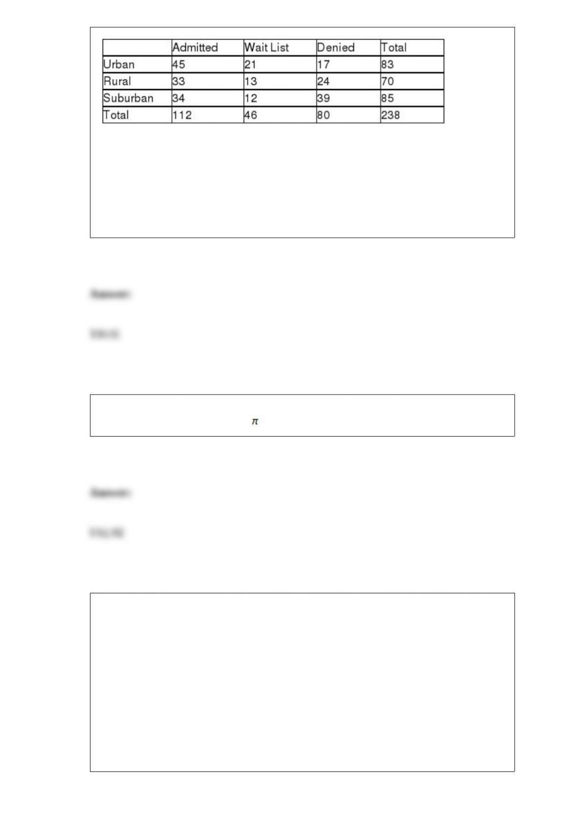
He will use this table to do a chi-square test of independence with a level of
significance of 0.01.
True or False: Referring to Table 12-11, the null hypothesis claims that “there is no
association between admission status at the college and the type of community in which
an applicant resides.”
True or False: As a general rule, one can use the normal distribution to approximate a
binomial distribution whenever n is at least 5.
TABLE 14-15
The superintendent of a school district wanted to predict the
percentage of students passing a sixth-grade proficiency test. She
obtained the data on percentage of students passing the proficiency
test (% Passing), mean teacher salary in thousands of dollars
(Salaries), and instructional spending per pupil in thousands of dollars
(Spending) of 47 schools in the state.
Following is the multiple regression output with Y = % Passing as the
dependent variable, X1 = Salaries and X2 = Spending:
True or False: Referring to Table 14-15, you can conclude definitively
that mean teacher salary individually has no impact on the mean
percentage of students passing the proficiency test, taking into
account the e.ect of instructional spending per pupil, at a 1% level of
significance based solely on but not actually computing the 99%
confidence interval estimate for β1.
True or False: TABLE 17-12
The marketing manager for a nationally franchised lawn service company would like to
study the characteristics that differentiate home owners who do and do not have a lawn
service. A random sample of 30 home owners located in a suburban area near a large
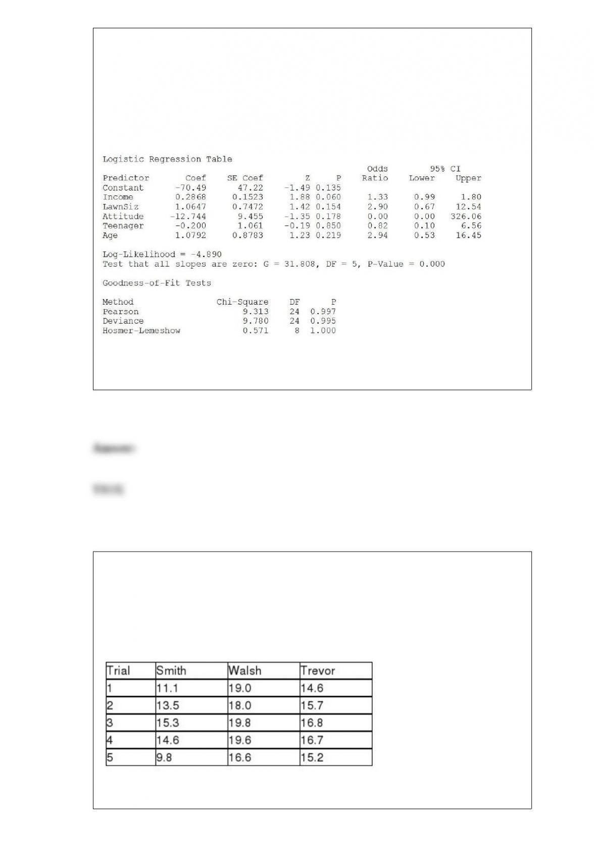
city was selected; 15 did not have a lawn service (code 0) and 15 had a lawn service
(code 1). Additional information available concerning these 30 home owners includes
family income (Income, in thousands of dollars), lawn size (Lawn Size, in thousands of
square feet), attitude toward outdoor recreational activities (Attitude 0 = unfavorable, 1
= favorable), number of teenagers in the household (Teenager), and age of the head of
the household (Age).
The Minitab output is given below:
Referring to Table 17-12, there is not enough evidence to conclude that Attitude makes
a significant contribution to the model in the presence of the other independent
variables at a 0.05 level of significance.
TABLE 11-4
An agronomist wants to compare the crop yield of 3 varieties of chickpea seeds. She
plants 15 fields, 5 with each variety. She then measures the crop yield in bushels per
acre. Treating this as a completely randomized design, the results are presented in the
table that follows.
True or False: Referring to Table 11-4, the null hypothesis should be rejected at 0.005
level of significance.
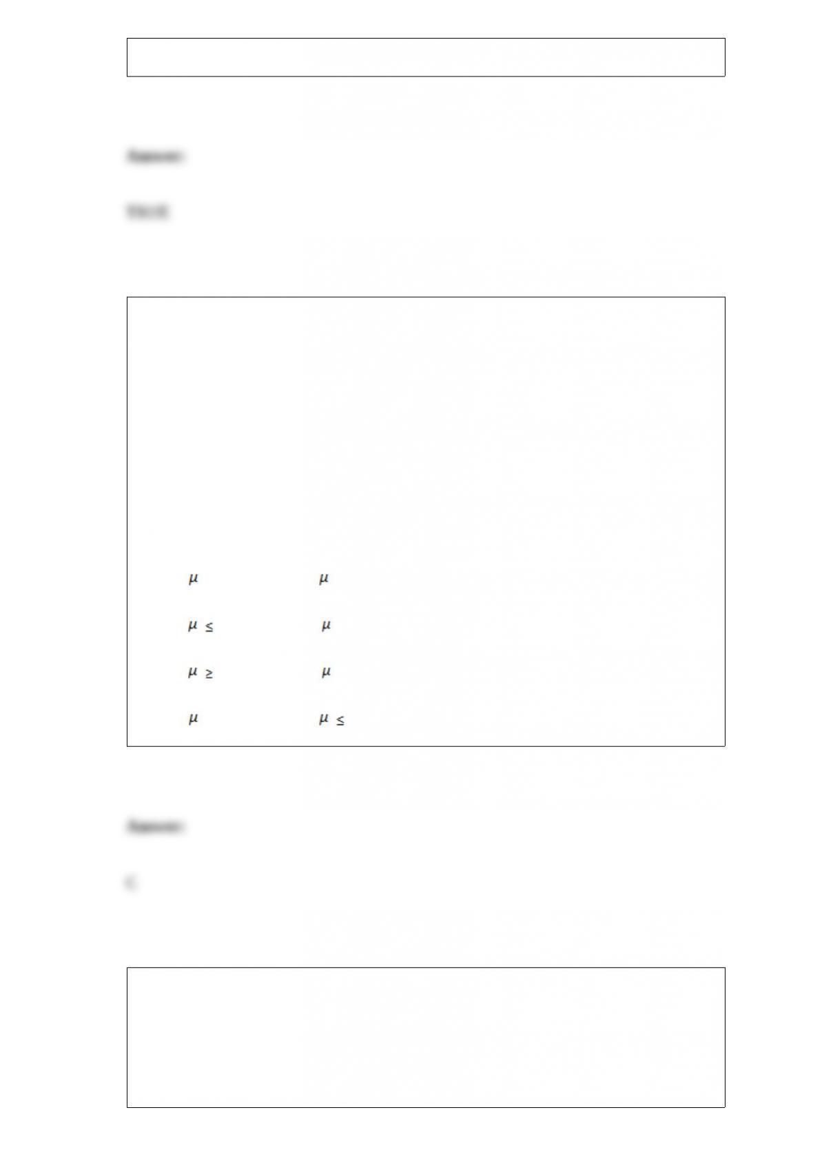
TABLE 9-4
A drug company is considering marketing a new local anesthetic. The effective time of
the anesthetic the drug company is currently producing has a normal distribution with a
mean of 7.4 minutes with a standard deviation of 1.2 minutes. The chemistry of the new
anesthetic is such that the effective time should be normally distributed with the same
standard deviation, but the mean effective time may be lower. If it is lower, the drug
company will market the new anesthetic; otherwise, they will continue to produce the
older one. A sample size of 36 results in a sample mean of 7.1. A hypothesis test will be
done to help make the decision.
Referring to Table 9-4, the appropriate hypotheses are
A) H0 : = 7.4 versus H1 : ≠7.4.
B) H0 : 7.4 versus H1 : > 7.4.
C) H0 : 7.4 versus H1 : < 7.4.
D) H0 : > 7.4 versus H1 : 7.4.
TABLE 13-11
A computer software developer would like to use the number of downloads (in
thousands) for the trial version of his new shareware to predict the amount of revenue
(in thousands of dollars) he can make on the full version of the new shareware.
Following is the output from a simple linear regression along with the residual plot and
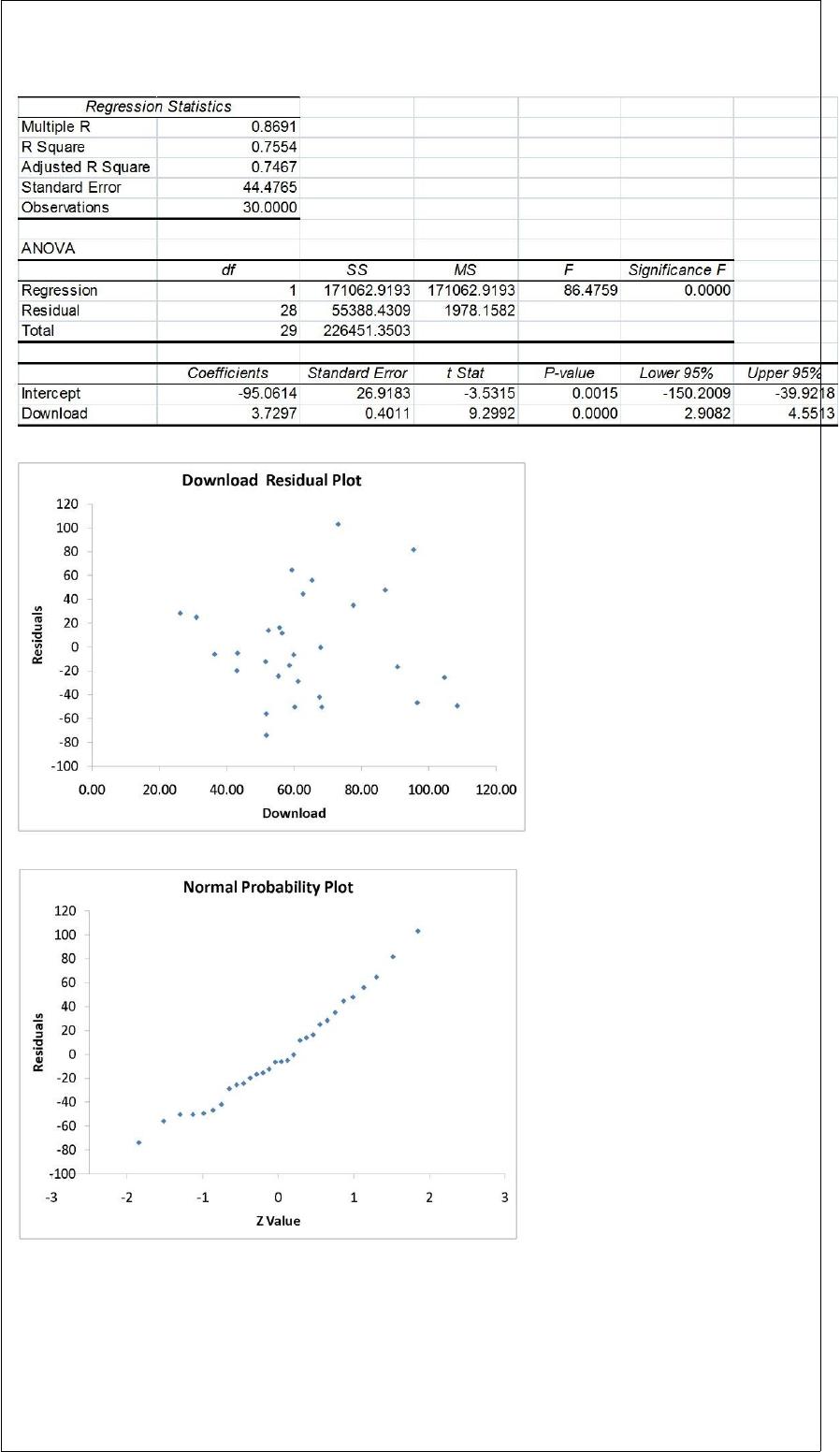
normal probability plot obtained from a data set of 30 different sharewares that he has
developed:
Referring to Table 13-11, which of the following assumptions appears to have been
violated?
A) Normality of error
B) Homoscedasticity
C) Independence of errors
D) None of the above.
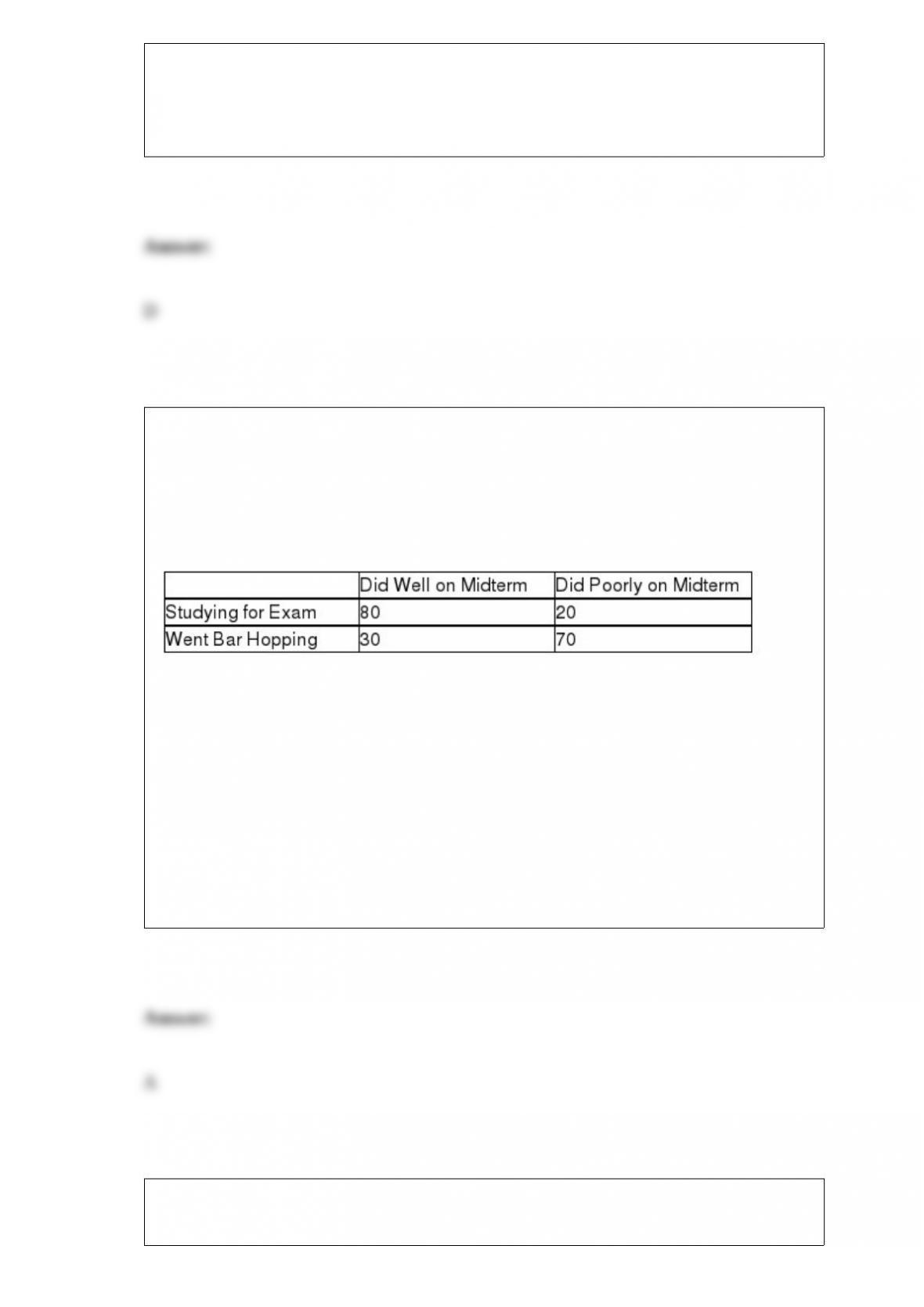
TABLE 4-2
An alcohol awareness task force at a Big-Ten university sampled 200 students after the
midterm to ask them whether they went bar hopping the weekend before the midterm or
spent the weekend studying, and whether they did well or poorly on the midterm. The
following result was obtained.
Referring to Table 4-2, what is the probability that a randomly selected student who
went bar hopping did well on the midterm?
A) 30/100 or 30%
B) 30/110 or 27.27%
C) 30/200 or 15%
D) (100/200) ∗ (110/200) or 27.50%
Assuming a linear relationship between X and Y, if the coefficient of correlation (r)
equals -0.30,
A) there is no correlation.
B) the slope (b1) is negative.
C) variable X is larger than variable Y.
D) the variance of X is negative.
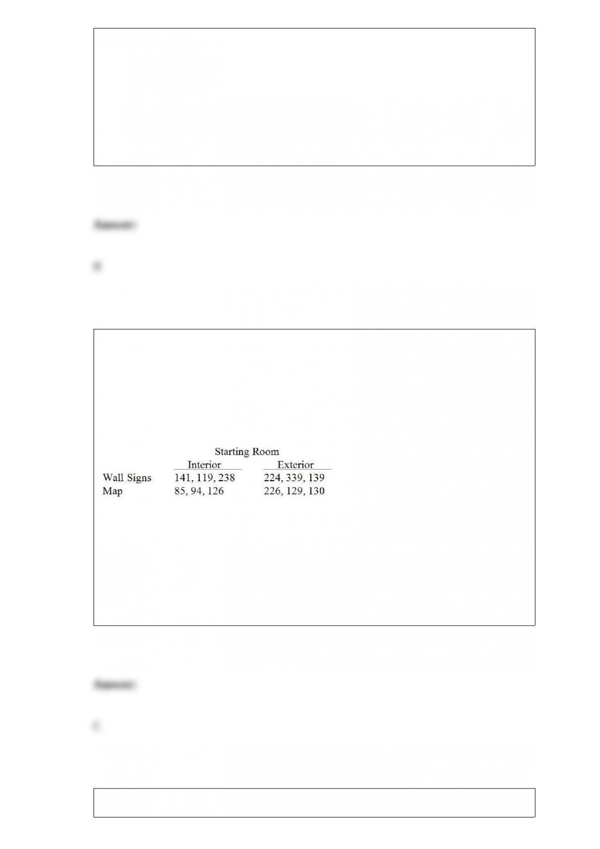
A campus researcher wanted to investigate the factors that affect visitor travel time in a
complex, multilevel building on campus. Specifically, he wanted to determine whether
different building signs (building maps versus wall signage) affect the total amount of
time visitors require to reach their destination and whether that time depends on
whether the starting location is inside or outside the building. Three subjects were
assigned to each of the combinations of signs and starting locations, and travel time in
seconds from beginning to destination was recorded. How should the data be analyzed?
A) completely randomized design
B) randomized block design
C) 2 x 2 factorial design
D) Levene’s test
TABLE 10-1
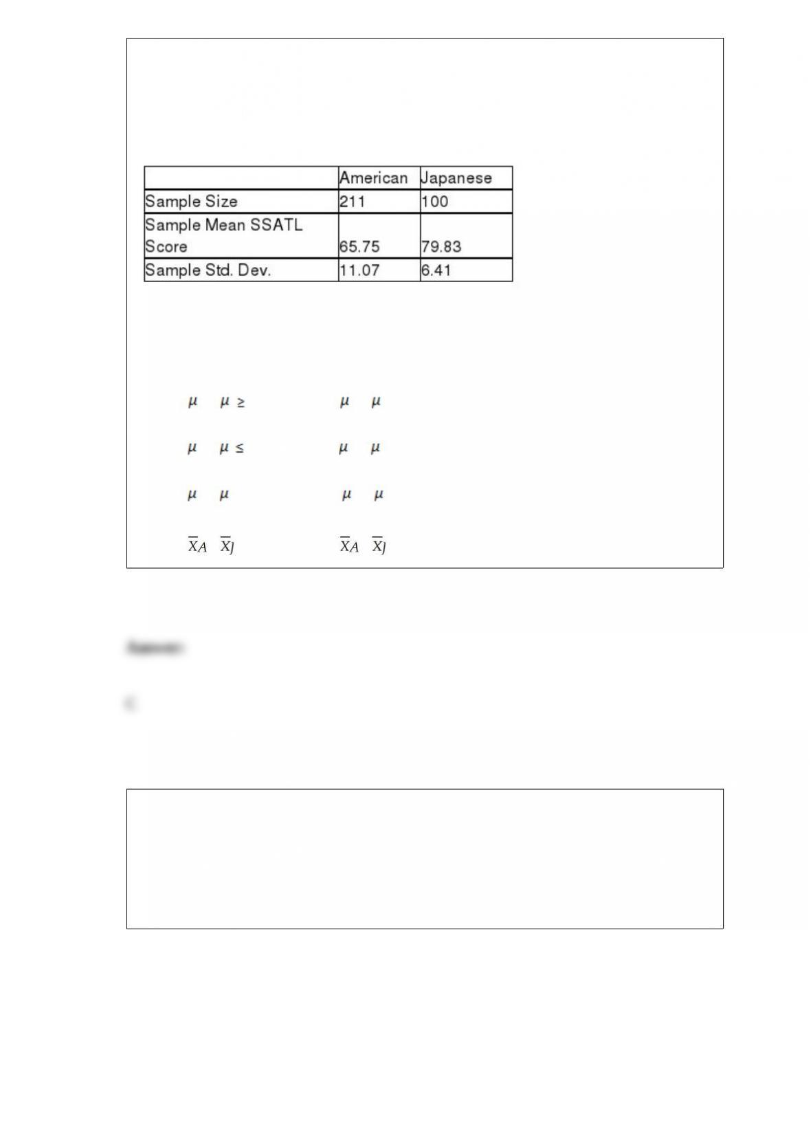
Are Japanese managers more motivated than American managers? A randomly selected
group of each were administered the Sarnoff Survey of Attitudes Toward Life (SSATL),
which measures motivation for upward mobility. The SSATL scores are summarized
below.
Referring to Table 10-1, give the null and alternative hypotheses to determine if the
mean SSATL score of Japanese managers differs from the mean SSATL score of
American managers.
A) H0 : A – J 0 versus H1 : A – J < 0
B) H0 : A – J 0 versus H1 : A – J > 0
C) H0 : A – J = 0 versus H1 : A – J ≠0
D) H0 : – = 0 versus H1 : – ≠0
TABLE 17-1
A real estate builder wishes to determine how house size (House) is influenced by
family income (Income), family size (Size), and education of the head of household
(School). House size is measured in hundreds of square feet, income is measured in
thousands of dollars, and education is in years. The builder randomly selected 50
families and ran the multiple regression. Microsoft Excel output is provided below:
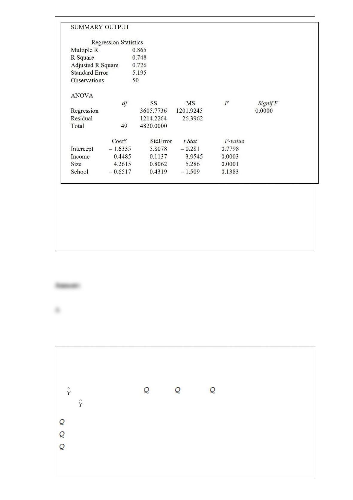
Referring to Table 17-1, what minimum annual income would an individual with a
family size of 9 and 10 years of education need to attain a predicted 5,000 square foot
home (House = 50)?
A) $44.14 thousand
B) $56.75 thousand
C) $178.33 thousand
D) $211.85 thousand
TABLE 16-14
A contractor developed a multiplicative time-series model to forecast the number of
contracts in future quarters, using quarterly data on number of contracts during the
3-year period from 2010 to 2012. The following is the resulting regression equation:
ln = 3.37 + 0.117 X – 0.083 1 + 1.28 2 + 0.617 3
where is the estimated number of contracts in a quarter
X is the coded quarterly value with X = 0 in the first quarter of 2010
1 is a dummy variable equal to 1 in the first quarter of a year and 0 otherwise
2 is a dummy variable equal to 1 in the second quarter of a year and 0 otherwise
3 is a dummy variable equal to 1 in the third quarter of a year and 0 otherwise
Referring to Table 16-14, to obtain a forecast for the first quarter of 2013 using the
model, which of the following sets of values should be used in the regression equation?
A) X = 12, 1 = 0, 2 = 0, 3 = 0
B) X = 12, 1 = 1, 2 = 0, 3 = 0
C) X = 13, 1 = 0, 2 = 0, 3 = 0
D) X = 13, 1 = 1, 2 = 0, 3 = 0
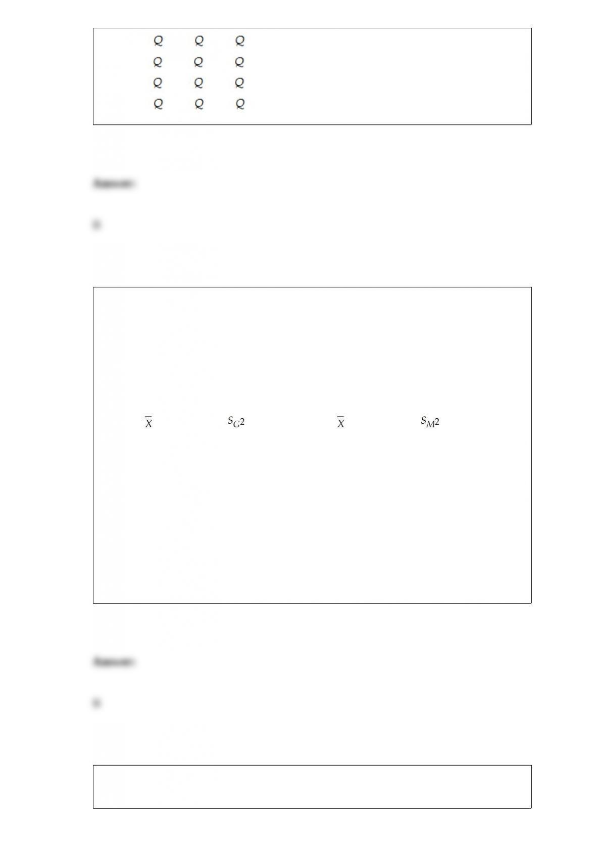
TABLE 10-3
A real estate company is interested in testing whether the mean time that families in
Gotham have been living in their current homes is less than families in Metropolis.
Assume that the two population variances are equal. A random sample of 100 families
from Gotham and a random sample of 150 families in Metropolis yield the following
data on length of residence in current homes.
Gotham: G = 35 months, = 900 Metropolis: M = 50 months, = 1050
Referring to Table 10-3, what is the test statistic for the difference between sample
means?
A) -8.75
B) -3.69
C) -2.33
D) -1.96
A major Blu-ray rental chain is considering opening a new store in an area that
currently does not have any such stores. The chain will open if there is evidence that
more than 5,000 of the 20,000 households in the area are equipped with Blu-ray
players. It conducts a telephone poll of 300 randomly selected households in the area
and finds that 96 have Blu-ray players. Which of the following tests will be the most
appropriate?
A) t test for the mean
B) Z test for the proportion
C) Pooled-variance t test
D) Separate-variance t test
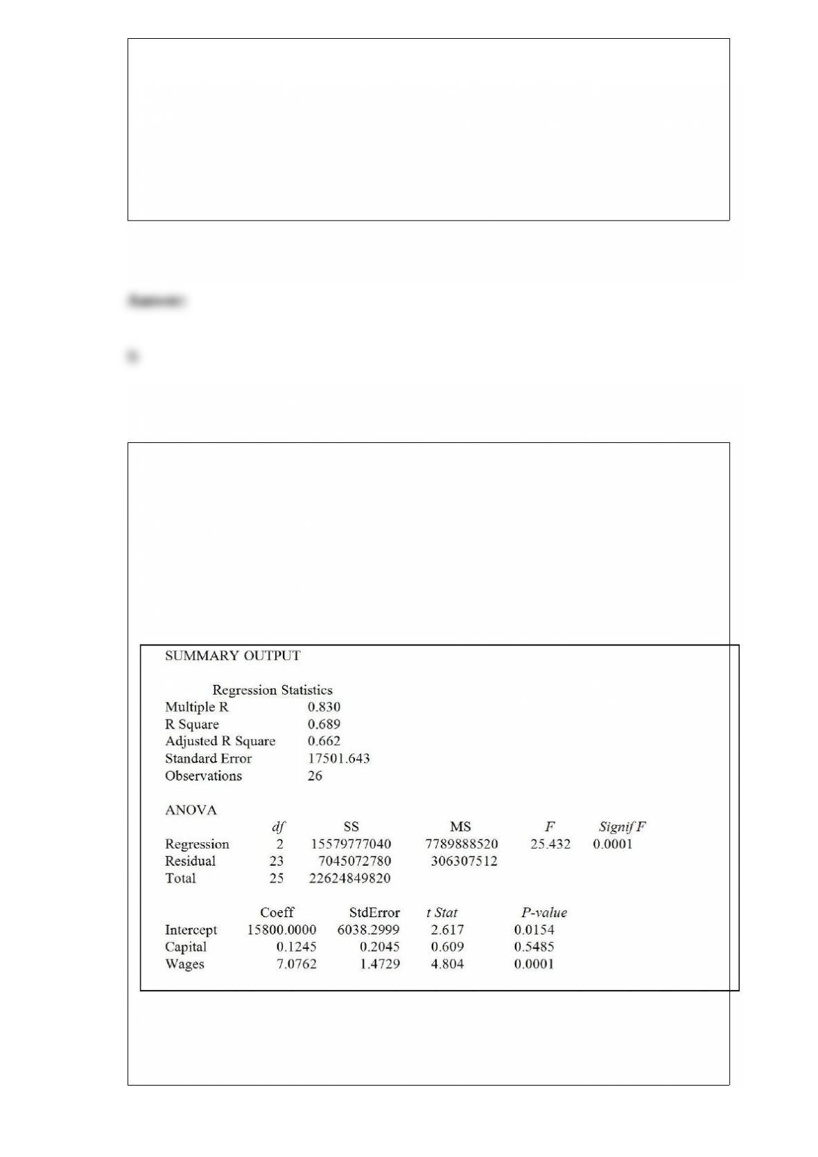
Referring to Table 14-5, one company in the sample had sales of $20 billion (Sales =
20,000). This company spent $300 million on capital and $700 million on wages. What
is the residual (in millions of dollars) for this data point?
TABLE 14-5
A microeconomist wants to determine how corporate sales are influenced by capital and
wage spending by companies. She proceeds to randomly select 26 large corporations
and record information in millions of dollars. The Microsoft Excel output below shows
results of this multiple regression.
A) 874.55
B) 622.87
C) -790.69
D) -983.56
The Dean of Students conducted a survey on campus. SAT score in mathematics is an
example of a ________ numerical variable.
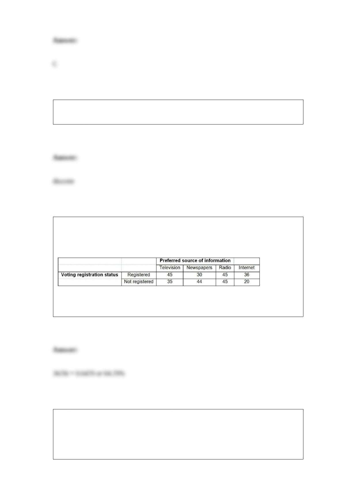
TABLE 4-11
A sample of 300 adults is selected. The contingency table below shows their registration
status and their preferred source of information on current events.
Referring to Table 4-11, what is the probability that an adult who prefers to get his/her
current information from the internet will be a registered voter?
TABLE 17-12
The marketing manager for a nationally franchised lawn service company would like to
study the characteristics that differentiate home owners who do and do not have a lawn
service. A random sample of 30 home owners located in a suburban area near a large
city was selected; 15 did not have a lawn service (code 0) and 15 had a lawn service
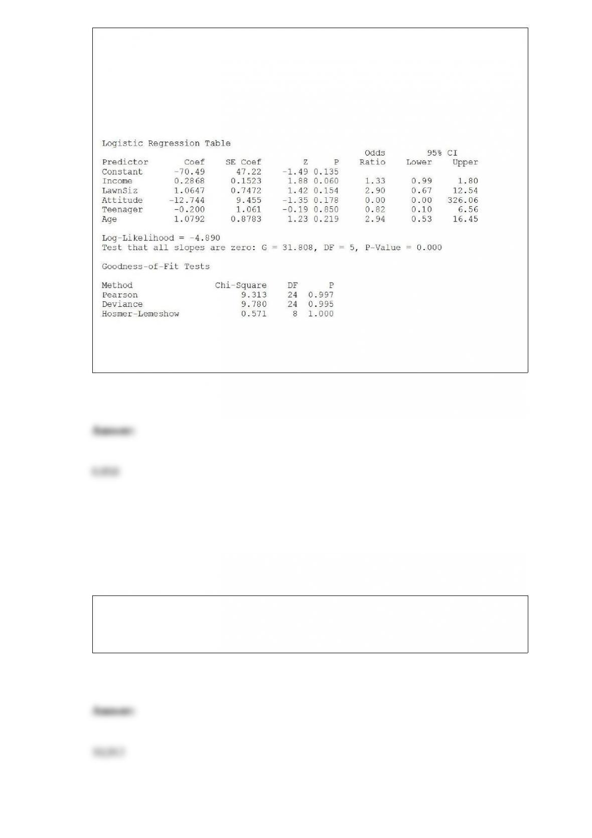
(code 1). Additional information available concerning these 30 home owners includes
family income (Income, in thousands of dollars), lawn size (Lawn Size, in thousands of
square feet), attitude toward outdoor recreational activities (Attitude 0 = unfavorable, 1
= favorable), number of teenagers in the household (Teenager), and age of the head of
the household (Age).
The Minitab output is given below:
Referring to Table 17-12, what is the p-value of the test statistic when testing whether
Teenager makes a significant contribution to the model in the presence of the other
independent variables?
A debate team of 4 is to be chosen from a class of 35. There are two twin brothers in the
class. How many possible ways can the team be formed which will include only one of
the twin brothers?
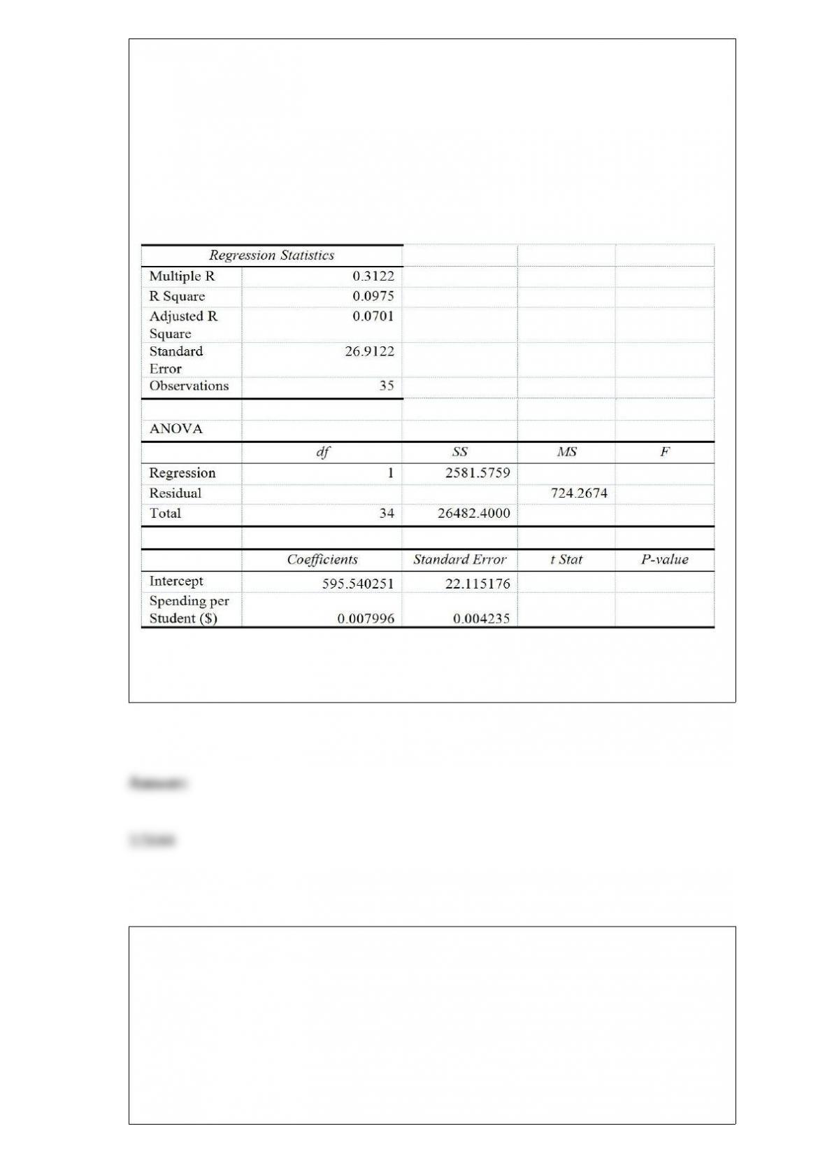
TABLE 13-13
In this era of tough economic conditions, voters increasingly ask the question: “Is the
educational achievement level of students dependent on the amount of money the state
in which they reside spends on education?” The partial computer output below is the
result of using spending per student ($) as the independent variable and composite score
which is the sum of the math, science and reading scores as the dependent variable on
35 states that participated in a study. The table includes only partial results.
Referring to Table 13-13, the value of the F test on whether spending per student affects
composite score is ________.
Referring to Table 14-7, the department head wants to test H0 : β1 =
β2 = 0. The value of the F-test statistic is ________.
TABLE 14-7
The department head of the accounting department wanted to see if
she could predict the GPA of students using the number of course
units (credits) and total SAT scores of each. She takes a sample of
students and generates the following Microsoft Excel output:
TABLE 17-10
Given below are results from the regression analysis where the dependent variable is
the number of weeks a worker is unemployed due to a layoff (Unemploy) and the
independent variables are the age of the worker (Age), the number of years of education
received (Edu), the number of years at the previous job (Job Yr), a dummy variable for
marital status (Married: 1 = married, 0 = otherwise), a dummy variable for head of
household (Head: 1 = yes, 0 = no) and a dummy variable for management position
(Manager: 1 = yes, 0 = no). We shall call this Model 1. The coefficient of partial
determination ( ) of each of the 6 predictors are, respectively,
0.2807, 0.0386, 0.0317, 0.0141, 0.0958, and 0.1201.
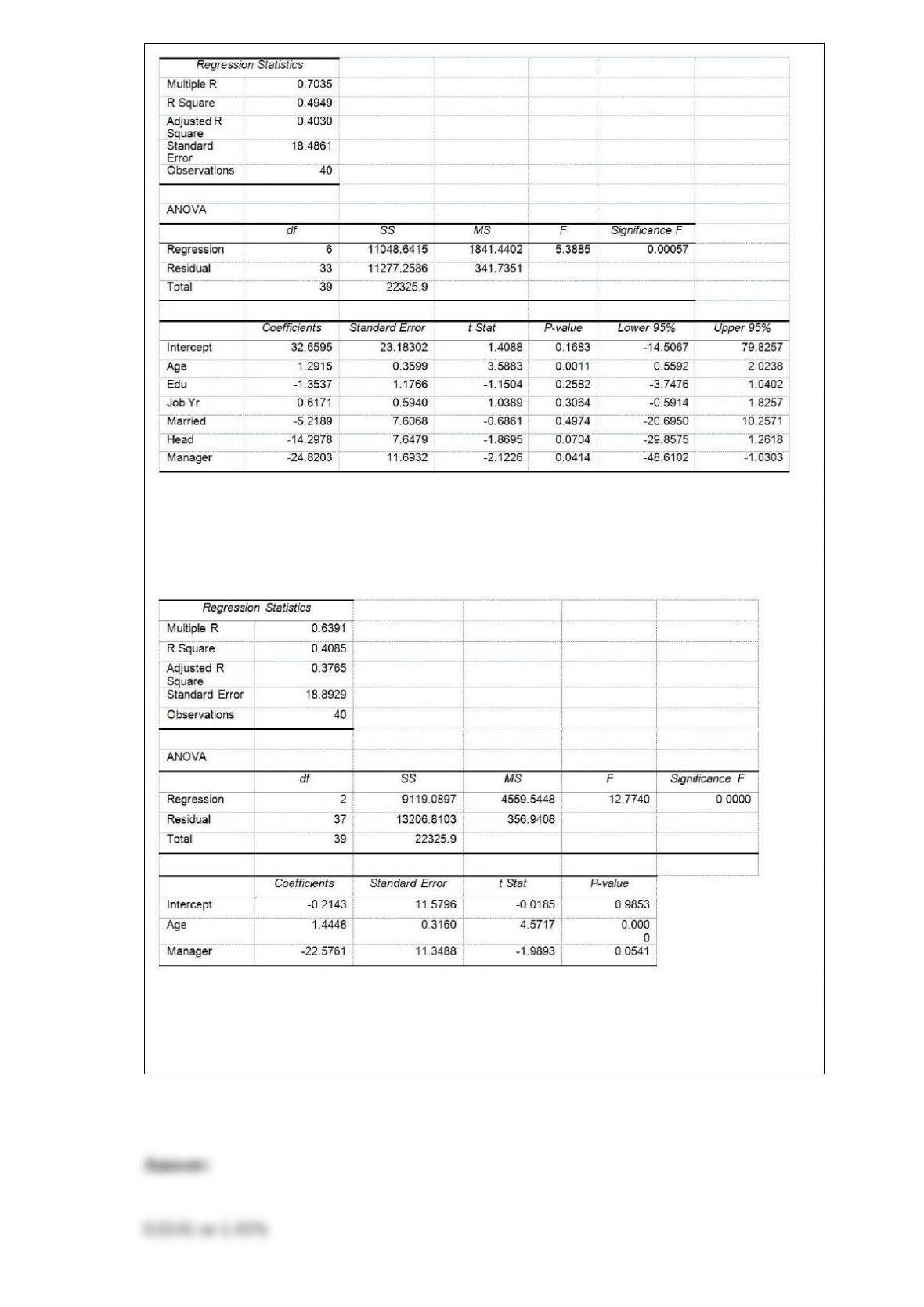
Model 2 is the regression analysis where the dependent variable is Unemploy and the
independent variables are Age and Manager. The results of the regression analysis are
given below:
Referring to Table 17-10, Model 1, ________ of the variation in the number of weeks a
worker is unemployed due to a layoff can be explained by the marital status while
controlling for the other independent variables.
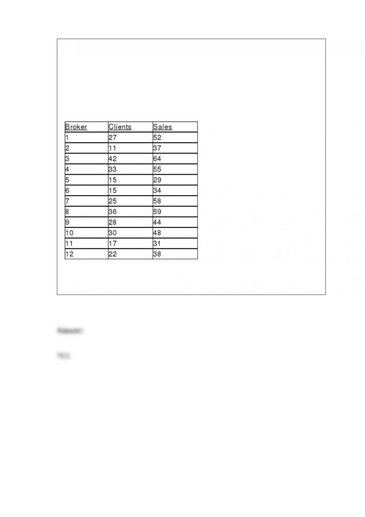
TABLE 13-4
The managers of a brokerage firm are interested in finding out if the number of new
clients a broker brings into the firm affects the sales generated by the broker. They
sample 12 brokers and determine the number of new clients they have enrolled in the
last year and their sales amounts in thousands of dollars. These data are presented in the
table that follows.
Referring to Table 13-4, ________% of the total variation in sales generated can be
explained by the number of new clients brought in.