TABLE 11-8
An important factor in selecting database software is the time required for a user to
learn how to use the system. To evaluate three potential brands (A, B and C) of database
software, a company designed a test involving five different employees. To reduce
variability due to differences among employees, each of the five employees is trained
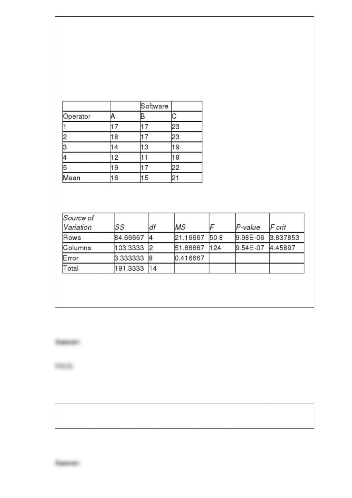
on each of the three different brands. The amount of time (in hours) needed to learn
each of the three different brands is given below:
Below is the Excel output for the randomized block design:
True or False: Referring to Table 11-8, the null hypothesis for the randomized block F
test for the difference in the means should be rejected at a 0.05 level of significance.
True or False: A completely randomized design with 4 groups would have 6 possible
pairwise comparisons.
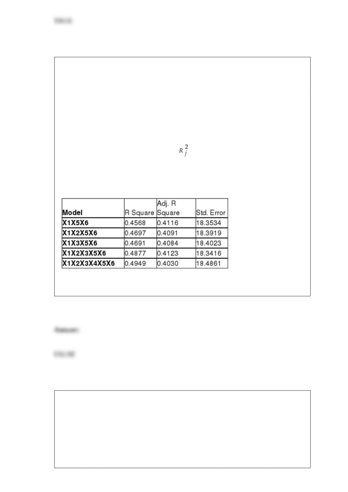
TABLE 15-6
Given below are results from the regression analysis on 40 observations where the
dependent variable is the number of weeks a worker is unemployed due to a layoff (Y)
and the independent variables are the age of the worker (X1), the number of years of
education received (X2), the number of years at the previous job (X3), a dummy variable
for marital status (X4: 1 = married, 0 = otherwise), a dummy variable for head of
household (X5: 1 = yes, 0 = no) and a dummy variable for management position (X6: 1
= yes, 0 = no).
The coefficient of multiple determination ( ) for the regression model using each of
the 6 variables Xj as the dependent variable and all other X variables as independent
variables are, respectively, 0.2628, 0.1240, 0.2404, 0.3510, 0.3342 and 0.0993.
The partial results from best-subset regression are given below:
True or False: Referring to Table 15-6, the variable X5 should be dropped to remove
collinearity.
True or False: TABLE 17-12
The marketing manager for a nationally franchised lawn service company would like to
study the characteristics that differentiate home owners who do and do not have a lawn
service. A random sample of 30 home owners located in a suburban area near a large
city was selected; 15 did not have a lawn service (code 0) and 15 had a lawn service
(code 1). Additional information available concerning these 30 home owners includes
family income (Income, in thousands of dollars), lawn size (Lawn Size, in thousands of
square feet), attitude toward outdoor recreational activities (Attitude 0 = unfavorable, 1
= favorable), number of teenagers in the household (Teenager), and age of the head of
the household (Age).
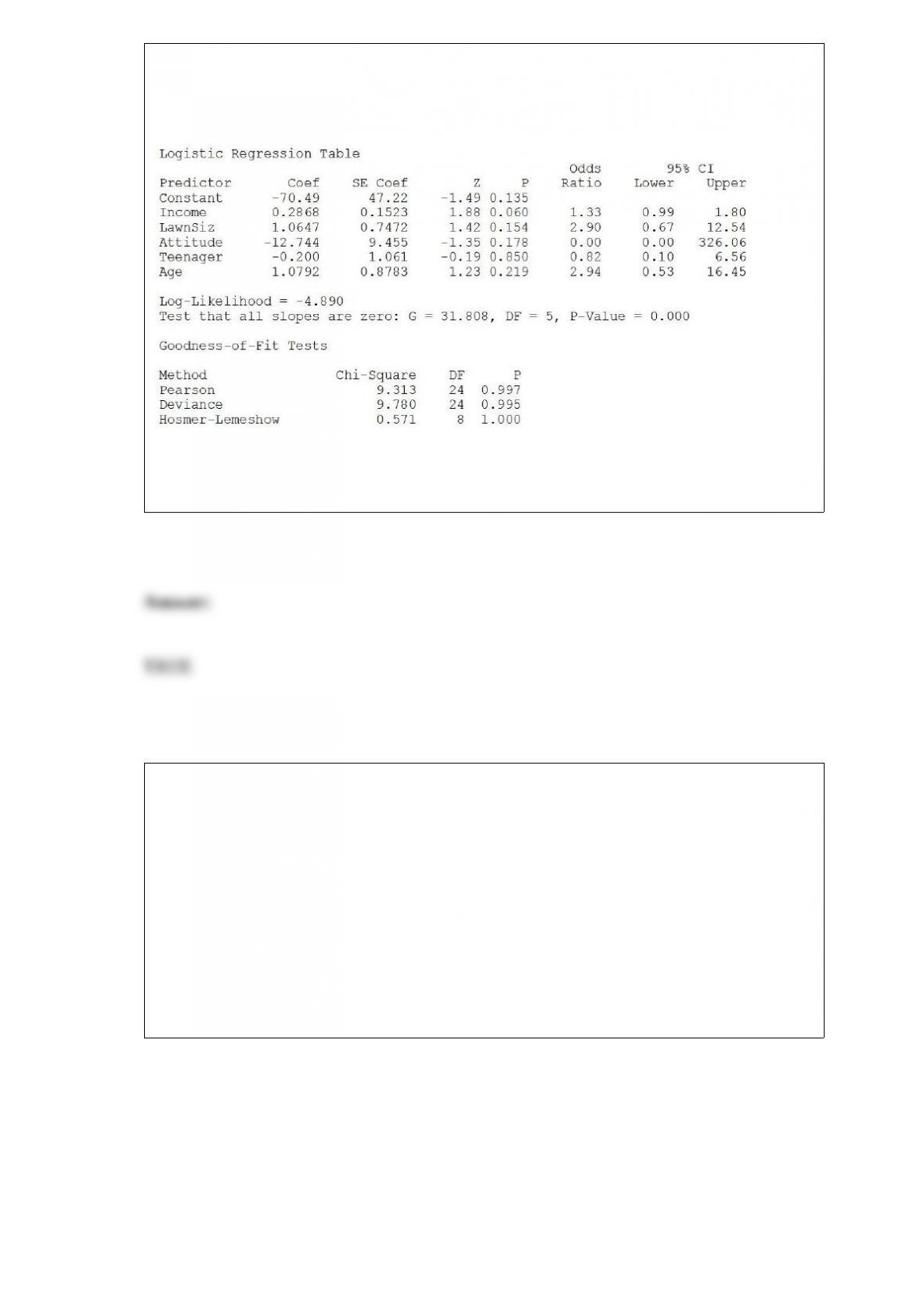
The Minitab output is given below:
Referring to Table 17-12, there is not enough evidence to conclude that LawnSize
makes a significant contribution to the model in the presence of the other independent
variables at a 0.05 level of significance.
True or False: TABLE 17-12
The marketing manager for a nationally franchised lawn service company would like to
study the characteristics that differentiate home owners who do and do not have a lawn
service. A random sample of 30 home owners located in a suburban area near a large
city was selected; 15 did not have a lawn service (code 0) and 15 had a lawn service
(code 1). Additional information available concerning these 30 home owners includes
family income (Income, in thousands of dollars), lawn size (Lawn Size, in thousands of
square feet), attitude toward outdoor recreational activities (Attitude 0 = unfavorable, 1
= favorable), number of teenagers in the household (Teenager), and age of the head of
the household (Age).
The Minitab output is given below:
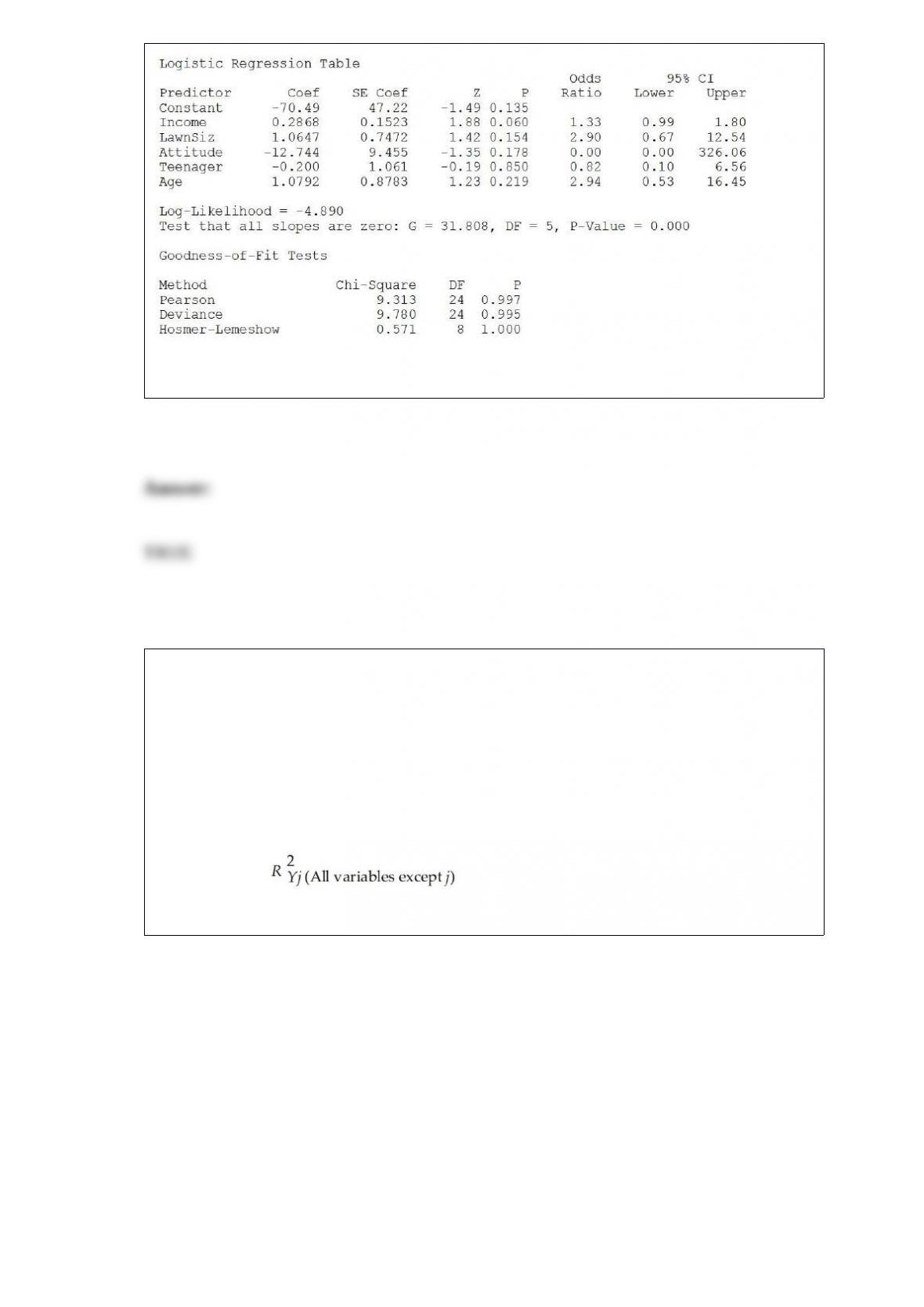
Referring to Table 17-12, the null hypothesis that the model is a good-fitting model
cannot be rejected when allowing for a 5% probability of making a type I error.
True or False: TABLE 17-10
Given below are results from the regression analysis where the dependent variable is
the number of weeks a worker is unemployed due to a layoff (Unemploy) and the
independent variables are the age of the worker (Age), the number of years of education
received (Edu), the number of years at the previous job (Job Yr), a dummy variable for
marital status (Married: 1 = married, 0 = otherwise), a dummy variable for head of
household (Head: 1 = yes, 0 = no) and a dummy variable for management position
(Manager: 1 = yes, 0 = no). We shall call this Model 1. The coefficient of partial
determination ( ) of each of the 6 predictors are, respectively,
0.2807, 0.0386, 0.0317, 0.0141, 0.0958, and 0.1201.
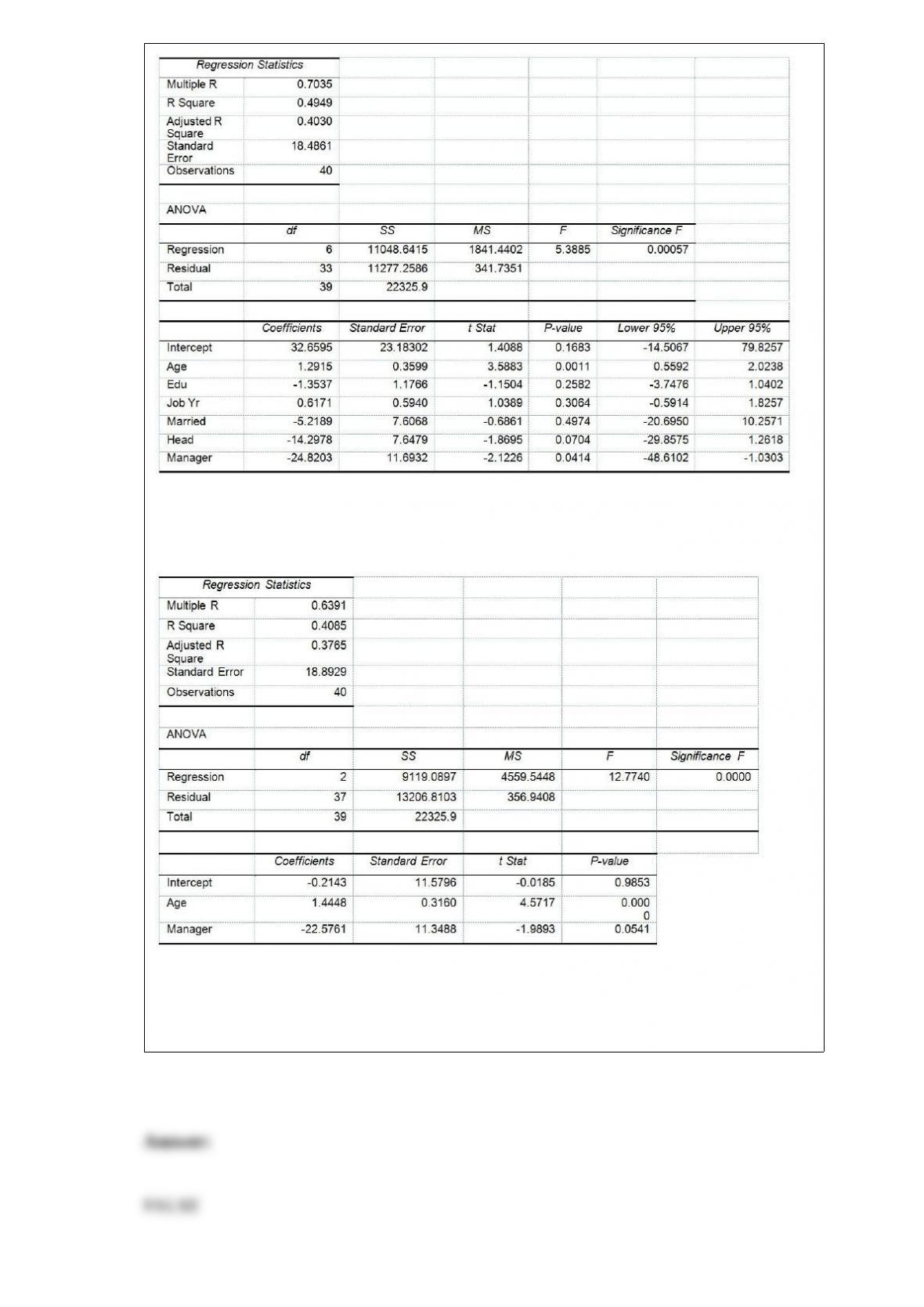
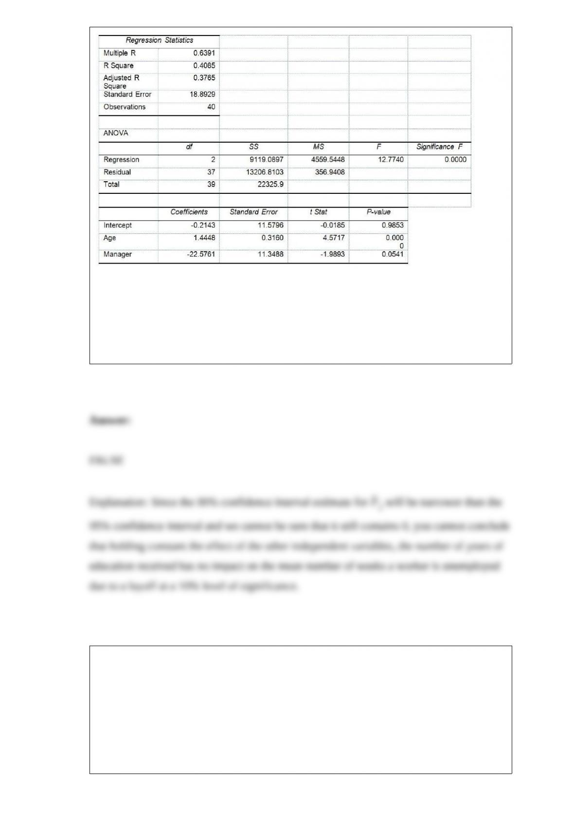
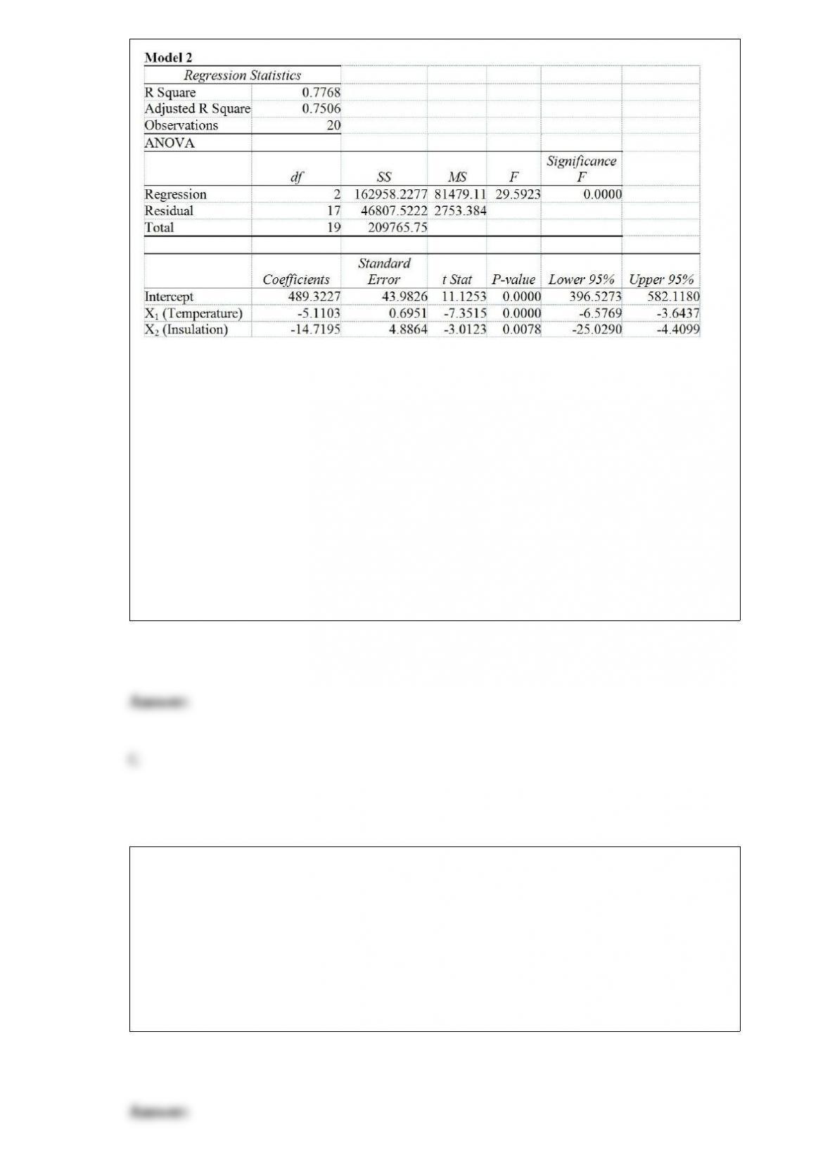
Model 2 is the regression analysis where the dependent variable is Unemploy and the
independent variables are Age and Manager. The results of the regression analysis are
given below:
Referring to Table 17-10 and using both Model 1 and Model 2, there is sufficient
evidence to conclude that at least one of the independent variables that are not
significant individually has become significant as a group in explaining the variation in
the dependent variable at a 5% level of significance.
True or False: A sample is the portion of the universe that is selected for analysis.
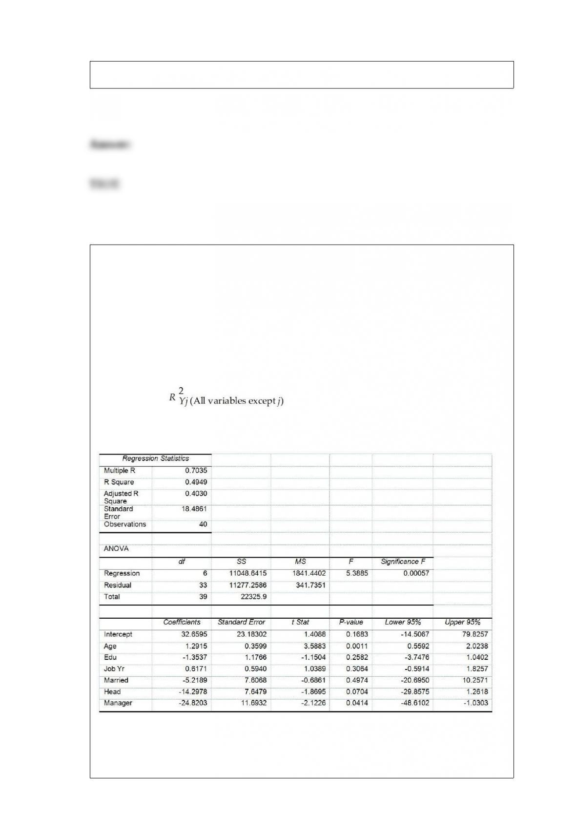
True or False: TABLE 17-10
Given below are results from the regression analysis where the dependent variable is
the number of weeks a worker is unemployed due to a layoff (Unemploy) and the
independent variables are the age of the worker (Age), the number of years of education
received (Edu), the number of years at the previous job (Job Yr), a dummy variable for
marital status (Married: 1 = married, 0 = otherwise), a dummy variable for head of
household (Head: 1 = yes, 0 = no) and a dummy variable for management position
(Manager: 1 = yes, 0 = no). We shall call this Model 1. The coefficient of partial
determination ( ) of each of the 6 predictors are, respectively,
0.2807, 0.0386, 0.0317, 0.0141, 0.0958, and 0.1201.
Model 2 is the regression analysis where the dependent variable is Unemploy and the
independent variables are Age and Manager. The results of the regression analysis are
given below:
Referring to Table 17-10, Model 1, we can conclude that, holding constant the effect of
the other independent variables, the number of years of education received has no
impact on the mean number of weeks a worker is unemployed due to a layoff at a 10%
level of significance if all we have is the information on the 95% confidence interval
estimate forβ2.
TABLE 8-3
To become an actuary, it is necessary to pass a series of 10 exams, including the most
important one, an exam in probability and statistics. An insurance company wants to
estimate the mean score on this exam for actuarial students who have enrolled in a
special study program. They take a sample of 8 actuarial students in this program and
determine that their scores are: 2, 5, 8, 8, 7, 6, 5, and 7. This sample will be used to
calculate a 90% confidence interval for the mean score for actuarial students in the
special study program.
True or False: Referring to Table 8-3, it is possible that the confidence interval obtained
will not contain the mean score for all actuarial students in the special study program.
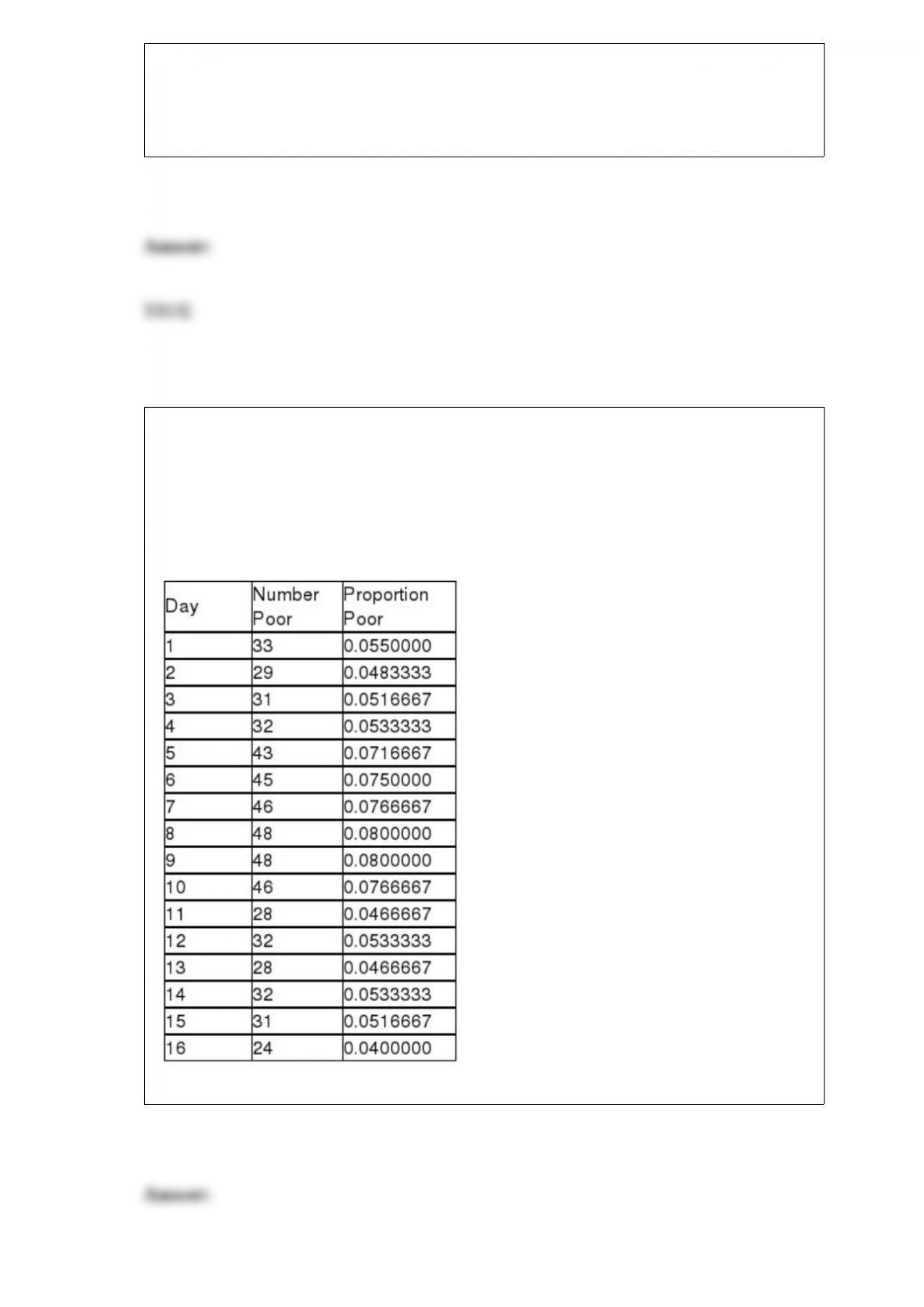
True or False: TABLE 18-6
The maker of a packaged candy wants to evaluate the quality of her production process.
On each of 16 consecutive days, she samples 600 bags of candy and determines the
number in each day’s sample that she considers to be of poor quality. The data that she
developed follow.
Referring to Table 18-6, the process seems to be in control.
True or False: Measurement error can become an ethical issue when a survey sponsor
chooses leading questions that guide the responses in a particular direction.
True or False: The chi-square test of independence requires that the expected frequency
in each cell to be at least 1.
A catalog company that receives the majority of its orders by telephone conducted a
study to determine how long customers were willing to wait on hold before ordering a
product. The length of waiting time was found to be a variable best approximated by an
exponential distribution with a mean length of waiting time equal to 2.8 minutes (i.e.
the mean number of calls answered in a minute is ). What proportion of callers is put
on hold longer than 2.8 minutes?
A) 0.3679
B) 0.50
C) 0.60810
D) 0.6321

TABLE 9-7
A major home improvement store conducted its biggest brand recognition campaign in
the company’s history. A series of new television advertisements featuring well-known
entertainers and sports figures were launched. A key metric for the success of television
advertisements is the proportion of viewers who “like the ads a lot”. A study of 1,189
adults who viewed the ads reported that 230 indicated that they “like the ads a lot.” The
percentage of a typical television advertisement receiving the “like the ads a lot” score
is believed to be 22%. Company officials wanted to know if there is evidence that the
series of television advertisements are less successful than the typical ad (i.e. if there is
evidence that the population proportion of “like the ads a lot” for the company’s ads is
less than 0.22) at a 0.01 level of significance.
Referring to Table 9-7, the parameter the company officials is interested in is
A) the mean number of viewers who “like the ads a lot.”
B) the total number of viewers who “like the ads a lot.”
C) the mean number of company officials who “like the ads a lot.”
D) the proportion of viewers who “like the ads a lot.”
A political pollster randomly selects a sample of 100 voters each day for 8 successive
days and asks how many will vote for the incumbent. The pollster wishes to see if the
percentage favoring the incumbent candidate is too erratic. Which of the following
would be the most appropriate analysis to perform?
A) Multiple linear regression
B) Exponential smoothing
C) Construct a p-chart
D) Perform a Levene’s test

Referring to Table 14-15, which of the following is the correct
alternative hypothesis to test whether instructional spending per
pupil has any effect on percentage of students passing the proficiency
test, taking into account the effect of mean teacher salary?
TABLE 14-15
The superintendent of a school district wanted to predict the
percentage of students passing a sixth-grade proficiency test. She
obtained the data on percentage of students passing the proficiency
test (% Passing), mean teacher salary in thousands of dollars
(Salaries), and instructional spending per pupil in thousands of dollars
(Spending) of 47 schools in the state.
Following is the multiple regression output with Y = % Passing as the
dependent variable, X1 = Salaries and X2 = Spending:
A) H1 : β0 ≠0
B) H1 : β1 ≠0
C) H1 : β2 ≠0
D) H1 : β3 ≠0
When extreme values are present in a set of data, which of the following descriptive
summary measures are most appropriate?
A) CV and range
B) arithmetic mean and standard deviation
C) interquartile range and median
D) variance and interquartile range
TABLE 18-3
A quality control analyst for a light bulb manufacturer is concerned that the time it takes
to produce a batch of light bulbs is too erratic. Accordingly, the analyst randomly
surveys 10 production periods each day for 14 days and records the sample mean and
range for each day.
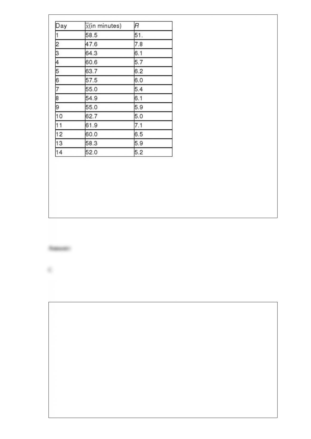
Referring to Table 18-3, suppose the analyst constructs an R chart to see if the
variability in production times is in-control. The R chart is characterized by which of
the following?
A) Increasing trend
B) Decreasing trend
C) In-control
D) Points outside the control limits
A physician and president of a Tampa Health Maintenance Organization (HMO) are
attempting to show the benefits of managed health care to an insurance company. The
physician believes that certain types of doctors are more cost-effective than others. To
investigate this, the president obtained independent random samples of 20 HMO
physicians from each of 4 primary specialties – General Practice (GP), Internal
Medicine (IM), Pediatrics (PED), and Family Physicians (FP) – and recorded the total
charges per member per month for each. A second variable which the president believes
influences total charges per member per month is whether the doctor is a foreign or
USA medical school graduate. To investigate this, the president also collected data on
20 foreign medical school graduates in each of the 4 primary specialty types described
above. Altogether, information on charges for 40 doctors (20 foreign and 20 USA
medical school graduates) was obtained for each of the 4 specialties. The president has
already found out that specialty types and origin of the medical degree do not interact to
affect the charges. Which of the following tests will be the most appropriate to find out
if the primary specialty affects the charges?
A) Tukey-Kramer multiple comparisons procedure for one-way ANOVA
B) One-way ANOVA F test for differences among more than two means
C) Two-way ANOVA F test for primary specialty effect
D) Two-way ANOVA F test for origin of the medical degree effect
A medical doctor is involved in a $1 million malpractice suit. He can either settle out of
court for $250,000 or go to court. If he goes to court and loses, he must pay $825,000
plus $175,000 in court costs. If he wins in court the plaintiffs pay the court costs.
Identify the actions of this decision-making problem.
A) Two choices: <1> go to court and <2> settle out of court.
B) Two possibilities: <1> win the case in court and <2> lose the case in court.
C) Four consequences resulting from Go/Settle and Win/Lose combinations.
D) The amount of money paid by the doctor.
Which of the following situations suggests a process that appears to be operating in a
state of statistical control?
A) A control chart with a series of consecutive points that are above the center line and
a series of consecutive points that are below the center line
B) A control chart in which no points fall outside either the upper control limit or the
lower control limit and no patterns are present
C) A control chart in which several points fall outside the upper control limit
D) All of the above
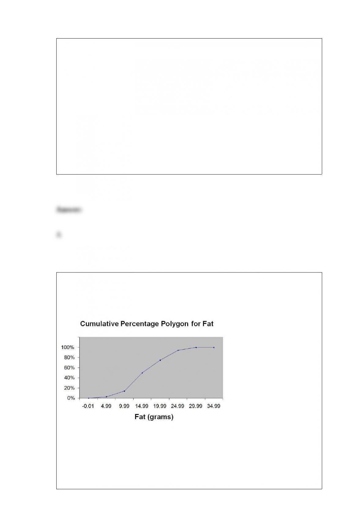
TABLE 17-4
You decide to predict gasoline prices in different cities and towns in the United States
for your term project. Your dependent variable is price of gasoline per gallon and your
explanatory variables are per capita income, the number of firms that manufacture
automobile parts in and around the city, the number of new business starts in the last
year, population density of the city, percentage of local taxes on gasoline, and the
number of people using public transportation. You collected data of 32 cities and
obtained a regression sum of squares SSR= 122.8821. Your computed value of standard
error of the estimate is 1.9549.
Referring to Table 17-4, the value of adjusted r2 is
A) 0.4576.
B) 0.5626.
C) 0.6472.
D) 95.5414.
TABLE 2-15
The figure below is the ogive for the amount of fat (in grams) for a sample of 36 pizza
products where the upper boundaries of the intervals are: 5, 10, 15, 20, 25, and 30.
Referring to Table 2-15, what percentage of pizza products contains between 10 and 25
grams of fat?
A) 14%
B) 44%

C) 62%
D) 81%
If we are testing for the difference between the means of 2 related populations with
samples of n1 = 20 and n2 = 20, the number of degrees of freedom is equal to
A) 39.
B) 38.
C) 19.
D) 18.
According to the Chebyshev rule, at least 75% of all observations in any data set are
contained within a distance of how many standard deviations around the mean?
A) 1
B) 2
C) 3
D) 4
A multiple-choice test has 30 questions. There are 4 choices for each question. A
student who has not studied for the test decides to answer all questions randomly. What
type of probability distribution can be used to figure out his chance of getting at least 20
questions right?
A) Binomial distribution
B) Poisson distribution
C) Hypergeometric distribution
D) None of the above.
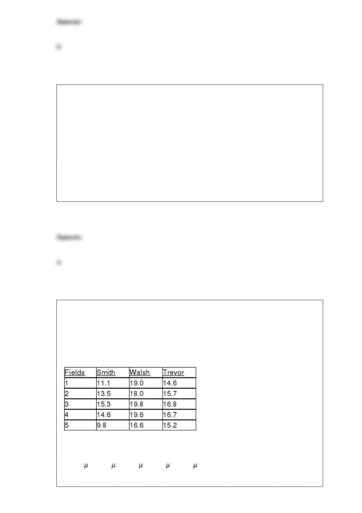
TABLE 11-10
An agronomist wants to compare the crop yield of 3 varieties of chickpea seeds. She
plants all 3 varieties of the seeds on each of 5 different patches of fields. She then
measures the crop yield in bushels per acre. Treating this as a randomized block design,
the results are presented in the table that follows.
Referring to Table 11-10, what is the null hypothesis for testing the block effects?
A) H0 : Field1 = Field2 = Field3 = Field4 = Field5
B) H0 : Smith = Walsh = Trevor
C) H0 : MField1 = MField2 = MField3 = MField4 = MField5
D) H0 : MSmith = MWalsh = MTrevor
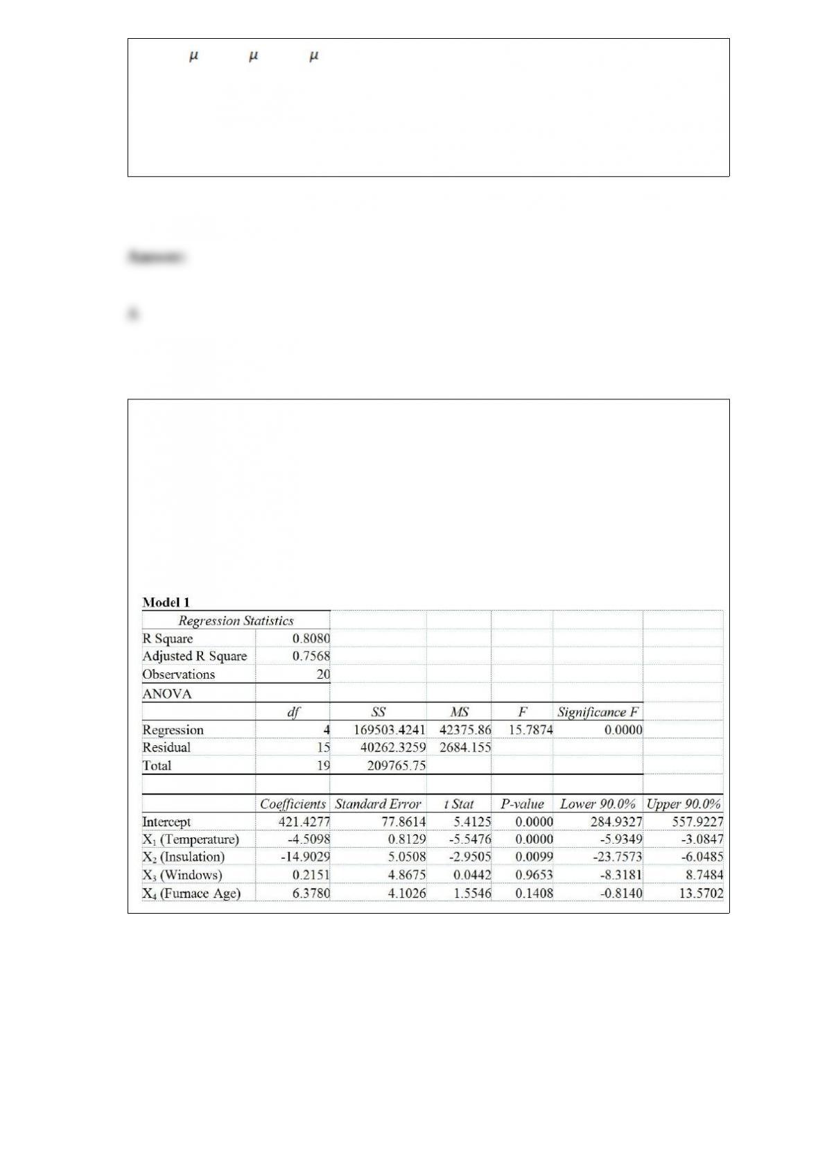
TABLE 17-2
One of the most common questions of prospective house buyers pertains to the cost of
heating in dollars (Y). To provide its customers with information on that matter, a large
real estate firm used the following 4 variables to predict heating costs: the daily
minimum outside temperature in degrees of Fahrenheit (X1), the amount of insulation in
inches (X2), the number of windows in the house (X3), and the age of the furnace in
years (X4). Given below are the EXCEL outputs of two regression models.
Referring to Table 17-2, what can we say about Model 1?
A) The model explains 77.7% of the sample variability of heating costs; after correcting
for the degrees of freedom, the model explains 75.1% of the sample variability of
heating costs.
B) The model explains 75.1% of the sample variability of heating costs; after correcting
for the degrees of freedom, the model explains 77.7% of the sample variability of
heating costs.
C) The model explains 80.8% of the sample variability of heating costs; after correcting
for the degrees of freedom, the model explains 75.7% of the sample variability of
heating costs.
D) The model explains 75.7% of the sample variability of heating costs; after correcting
for the degrees of freedom, the model explains 80.8% of the sample variability of
heating costs.
TABLE 4-4
Suppose that patrons of a restaurant were asked whether they preferred water or
whether they preferred soda. 70% said that they preferred water. 60% of the patrons
were male. 80% of the males preferred water.
Referring to Table 4-4, suppose a randomly selected patron is a female. Then the
probability that the patron prefers water is ________.

Referring to Table 14-15, what is the value of the test statistic when
testing whether mean teacher salary has any effect on percentage of
students passing the proficiency test, taking into account the effect of
instructional spending per pupil?
TABLE 14-15
The superintendent of a school district wanted to predict the
percentage of students passing a sixth-grade proficiency test. She
obtained the data on percentage of students passing the proficiency
test (% Passing), mean teacher salary in thousands of dollars
(Salaries), and instructional spending per pupil in thousands of dollars
(Spending) of 47 schools in the state.
Following is the multiple regression output with Y = % Passing as the
dependent variable, X1 = Salaries and X2 = Spending:
If X has a binomial distribution with n = 4 and p = 0.3, then P(X > 1) = ________.
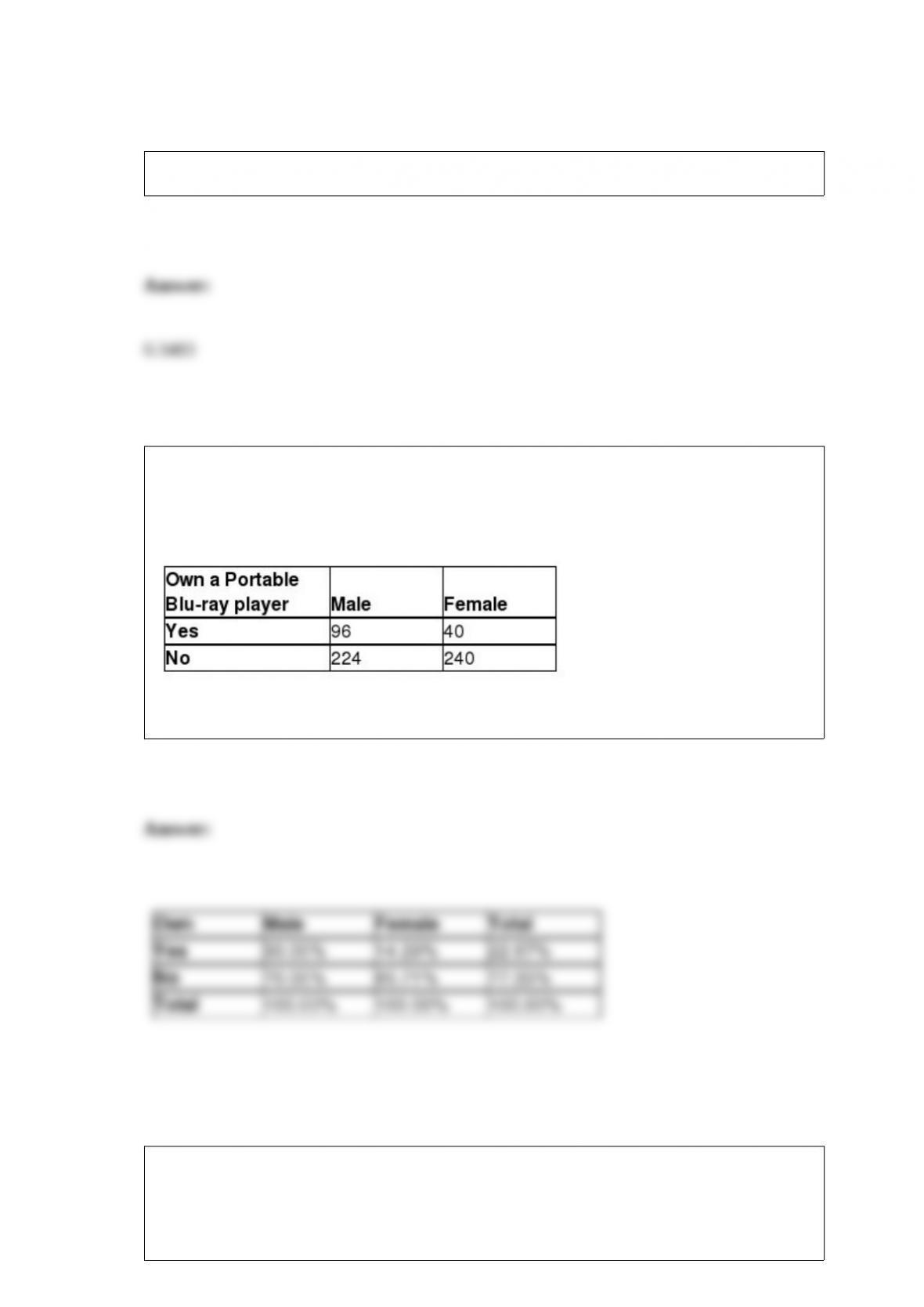
TABLE 2-14
The table below contains the number of people who own a portable Blu-ray player in a
sample of 600 broken down by gender.
Referring to Table 2-14, construct a table of column percentages.
Referring to Table 14-15, what are the lower and upper limits of the
95% confidence interval estimate for the effect of a one thousand
dollar increase in mean teacher salary on the mean percentage of
students passing the proficiency test?

TABLE 14-15
The superintendent of a school district wanted to predict the
percentage of students passing a sixth-grade proficiency test. She
obtained the data on percentage of students passing the proficiency
test (% Passing), mean teacher salary in thousands of dollars
(Salaries), and instructional spending per pupil in thousands of dollars
(Spending) of 47 schools in the state.
Following is the multiple regression output with Y = % Passing as the
dependent variable, X1 = Salaries and X2 = Spending:
TABLE 15-4
The superintendent of a school district wanted to predict the percentage of students
passing a sixth-grade proficiency test. She obtained the data on percentage of students
passing the proficiency test (% Passing), daily mean of the percentage of students
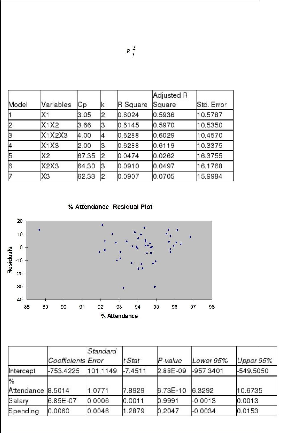
attending class (% Attendance), mean teacher salary in dollars (Salaries), and
instructional spending per pupil in dollars (Spending) of 47 schools in the state.
Let Y = % Passing as the dependent variable, X1 = % Attendance, X2 = Salaries and X3
= Spending.
The coefficient of multiple determination ( ) of each of the 3 predictors with all the
other remaining predictors are, respectively, 0.0338, 0.4669, and 0.4743.
The output from the best-subset regressions is given below:
Following is the residual plot for % Attendance:
Following is the output of several multiple regression models:
Model (I):
Model (II):
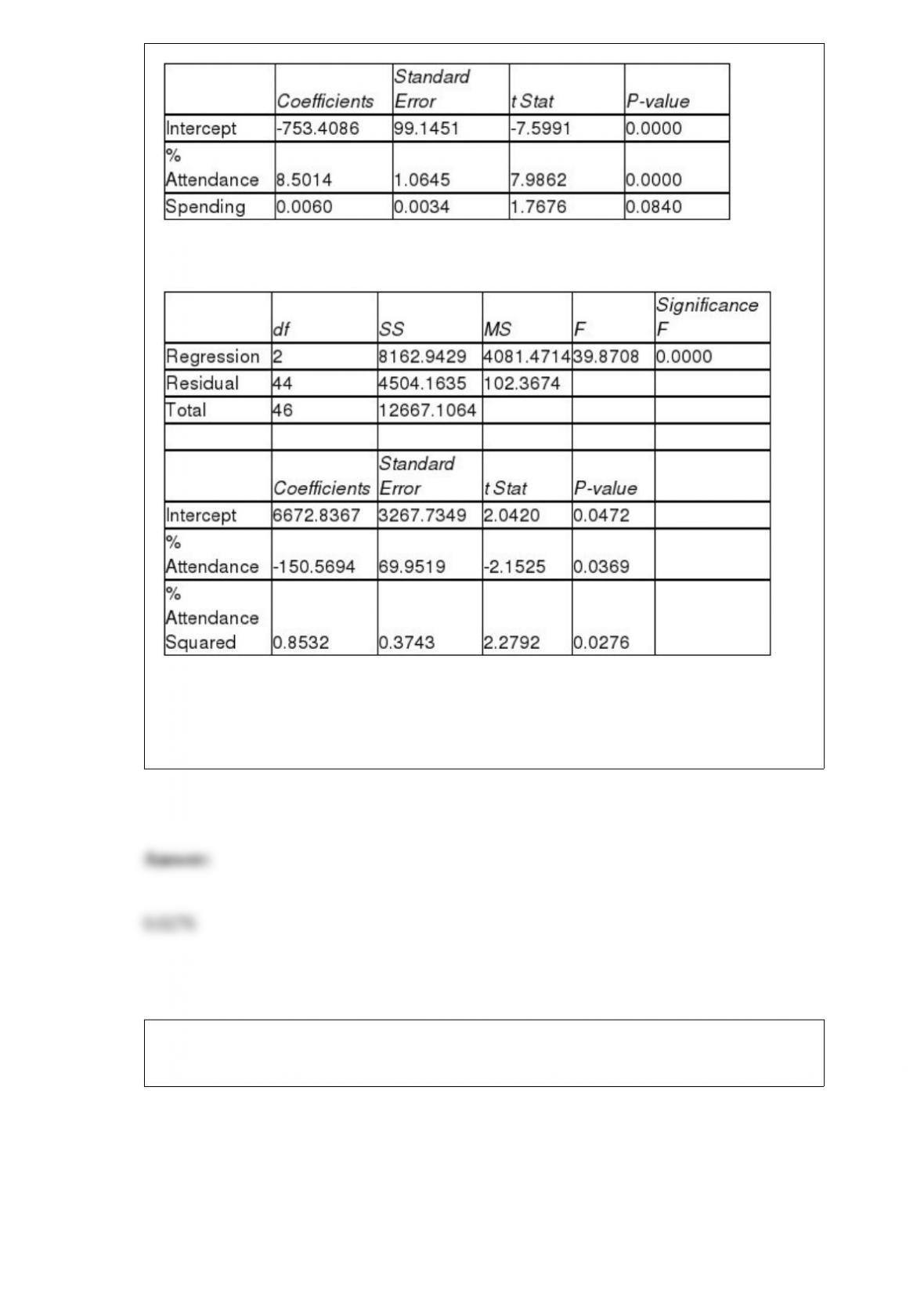
Model (III):
Referring to Table 15-4, what is the p-value of the test statistic to determine whether the
quadratic effect of daily average of the percentage of students attending class on
percentage of students passing the proficiency test is significant at a 5% level of
significance?
TABLE 16-16
Given below are the prices of a basket of four food items from 2008 to 2012.
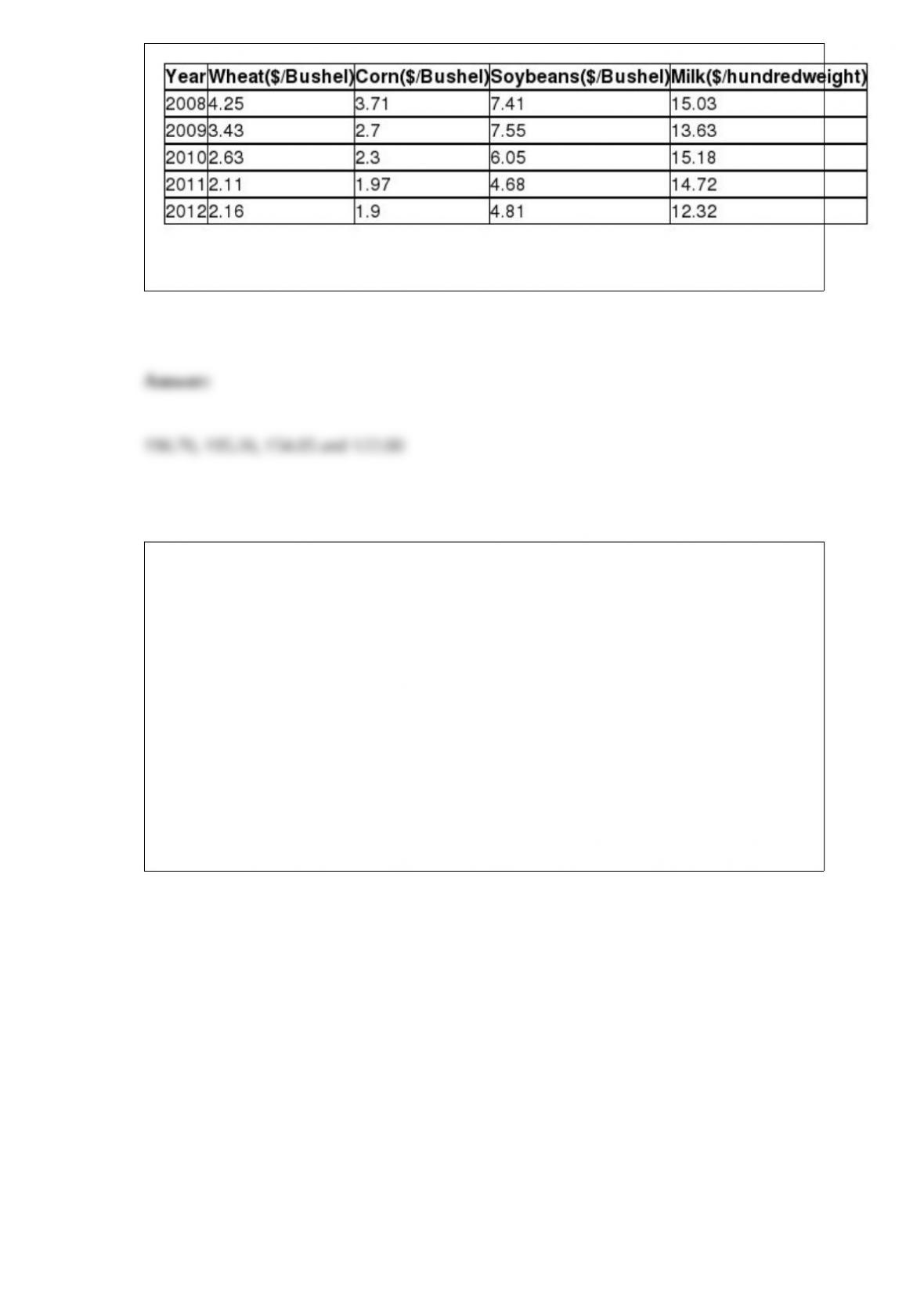
Referring to Table 16-16, what are the simple price indices for wheat, corn, soybeans
and milk, respectively, in 2008 using 2012 as the base year?
Referring to Table 14-8, the partial F test for
H0 : Variable X2 does not significantly improve the model after
variable X1 has been included
H1 Variable X2 significantly improves the model after variable X1 has
been included
has ________ and ________ degrees of freedom.TABLE 14-8
A financial analyst wanted to examine the relationship between salary
(in $1,000) and 2 variables: age
(X1 = Age) and experience in the field (X2 = Exper). He took a sample
of 20 employees and obtained the following Microsoft Excel output:

Also, the sum of squares due to the regression for the model that
includes only Age is 5022.0654 while the sum of squares due to the
regression for the model that includes only Exper is 125.9848.
The amount of tea leaves in a can from a particular production line is normally
distributed with = 110 grams and = 25 grams. A sample of 25 cans is to be selected.
So, the middle 70% of all sample means will fall between what two values?

TABLE 14-15
The superintendent of a school district wanted to predict the
percentage of students passing a sixth-grade proficiency test. She
obtained the data on percentage of students passing the proficiency
test (% Passing), mean teacher salary in thousands of dollars
(Salaries), and instructional spending per pupil in thousands of dollars
(Spending) of 47 schools in the state.
Following is the multiple regression output with Y = % Passing as the
dependent variable, X1 = Salaries and X2 = Spending:
Referring to Table 14-15, what are the numerator and denominator
degrees of freedom, respectively, for the test statistic to determine
whether there is a significant relationship between percentage of
students passing the proficiency test and the entire set of explanatory
variables?
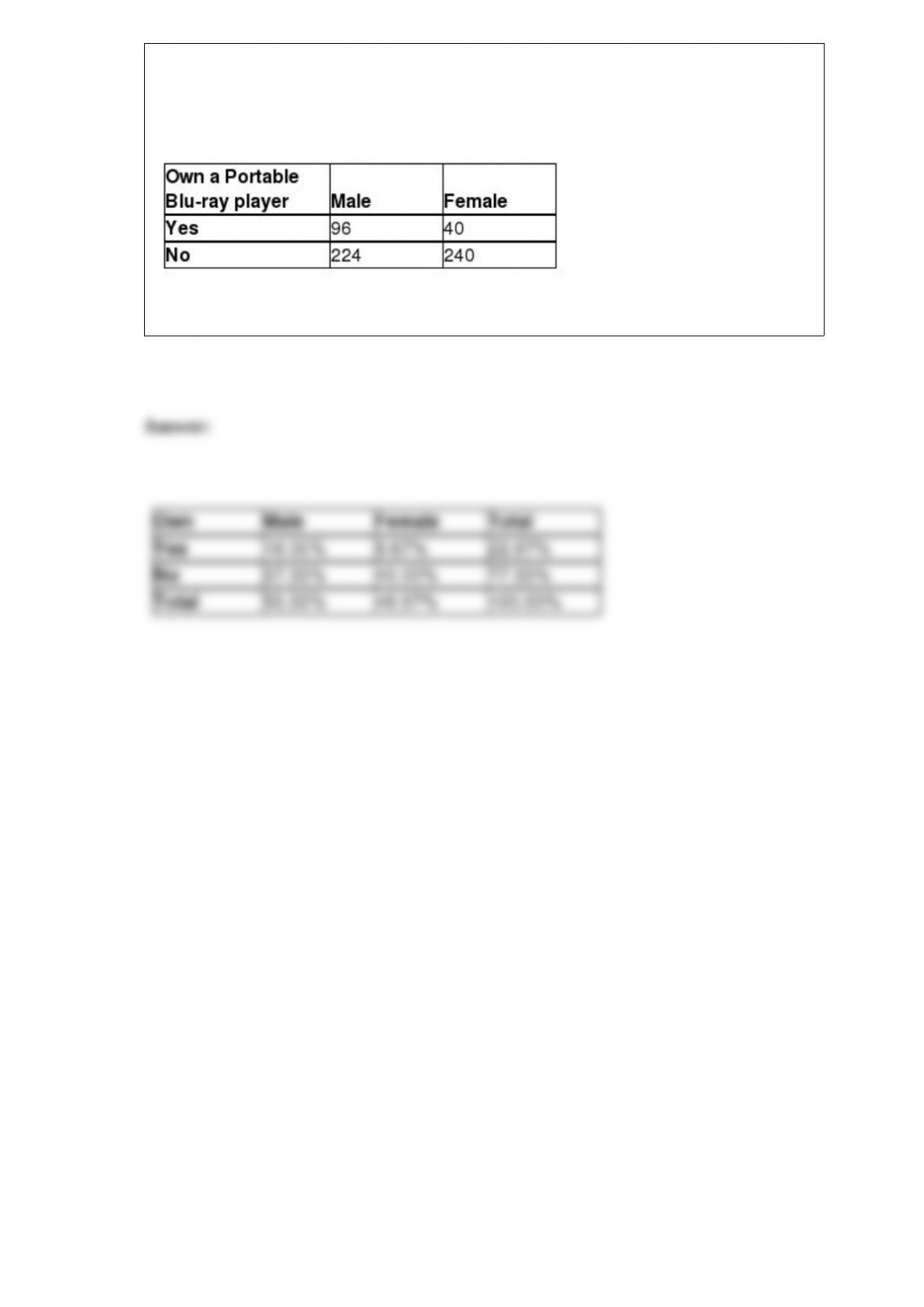
TABLE 2-14
The table below contains the number of people who own a portable Blu-ray player in a
sample of 600 broken down by gender.
Referring to Table 2-14, construct a table of total percentages.