True or False: TABLE 17-8
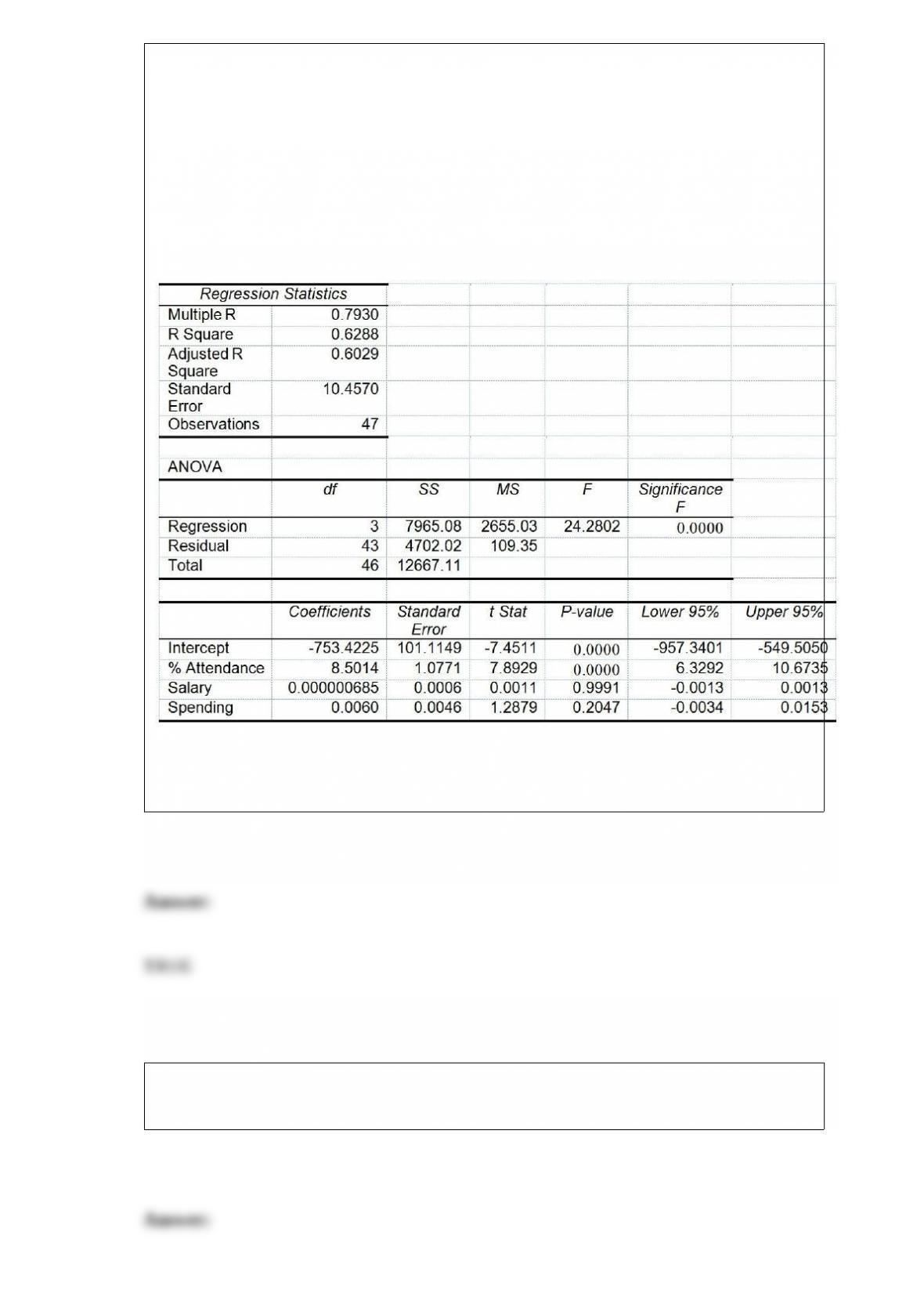
The superintendent of a school district wanted to predict the percentage of students
passing a sixth-grade proficiency test. She obtained the data on percentage of students
passing the proficiency test (% Passing), daily mean of the percentage of students
attending class (% Attendance), mean teacher salary in dollars (Salaries), and
instructional spending per pupil in dollars (Spending) of 47 schools in the state.
Following is the multiple regression output with Y = % Passing as the dependent
variable, X1 = % Attendance, X2 = Salaries and X3 = Spending:
Referring to Table 17-8, the null hypothesis H0 : β1 = β2 = β3 = 0 implies that the
percentage of students passing the proficiency test is not affected by any of the
explanatory variables.
True or False: The number of males selected in a sample of 5 students taken without
replacement from a class of 9 females and 18 males has a hypergeometric distribution.
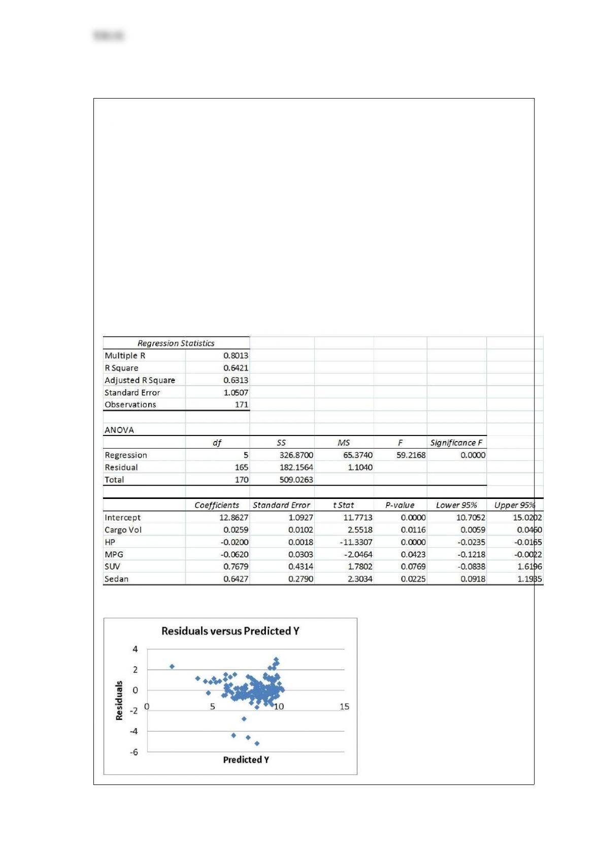
True or False: TABLE 17-9
What are the factors that determine the acceleration time (in sec.) from 0 to 60 miles per
hour of a car? Data on the following variables for 171 different vehicle models were
collected:
Accel Time: Acceleration time in sec.
Cargo Vol: Cargo volume in cu. ft.
HP: Horsepower
MPG: Miles per gallon
SUV: 1 if the vehicle model is an SUV with Coupe as the base when SUV and Sedan
are both 0
Sedan: 1 if the vehicle model is a sedan with Coupe as the base when SUV and Sedan
are both 0
The regression results using acceleration time as the dependent variable and the
remaining variables as the independent variables are presented below.
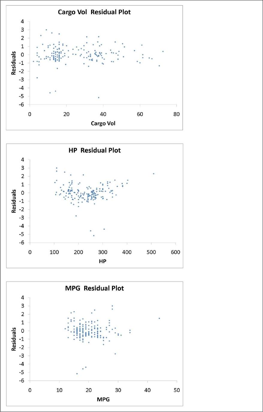
The various residual plots are as shown below.
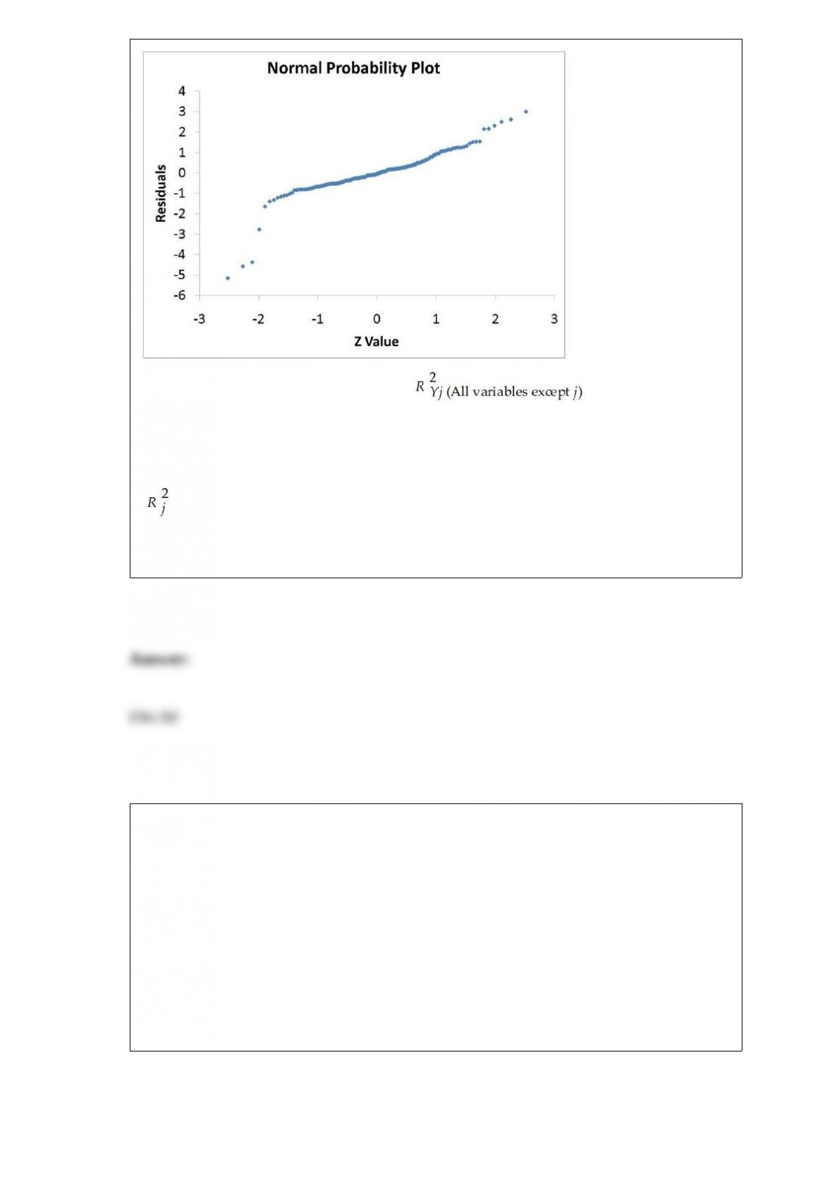
The coefficient of partial determination ( ) of each of the 5
predictors are, respectively, 0.0380, 0.4376, 0.0248, 0.0188, and 0.0312.
The coefficient of multiple determination for the regression model using each of the 5
variables Xj as the dependent variable and all other X variables as independent variables
( ) are, respectively, 0.7461, 0.5676, 0.6764, 0.8582, 0.6632.
Referring to Table 17-9, the 0 to 60 miles per hour acceleration time of a sedan is
predicted to be 0.7679 seconds higher than that of an SUV.
TABLE 12-20
A filling machine at a local soft drinks company is calibrated to fill the cans at a mean
amount of 12 fluid ounces and a standard deviation of 0.5 ounces. The company wants
to test whether the standard deviation of the amount filled by the machine is 0.5 ounces.
A random sample of 15 cans filled by the machine reveals a standard deviation of 0.67
ounces.
True or False: Referring to Table 12-20, there is sufficient evidence to conclude that the
standard deviation of the amount filled by the machine is not exactly 0.5 ounces when
using a 10% level of significance.
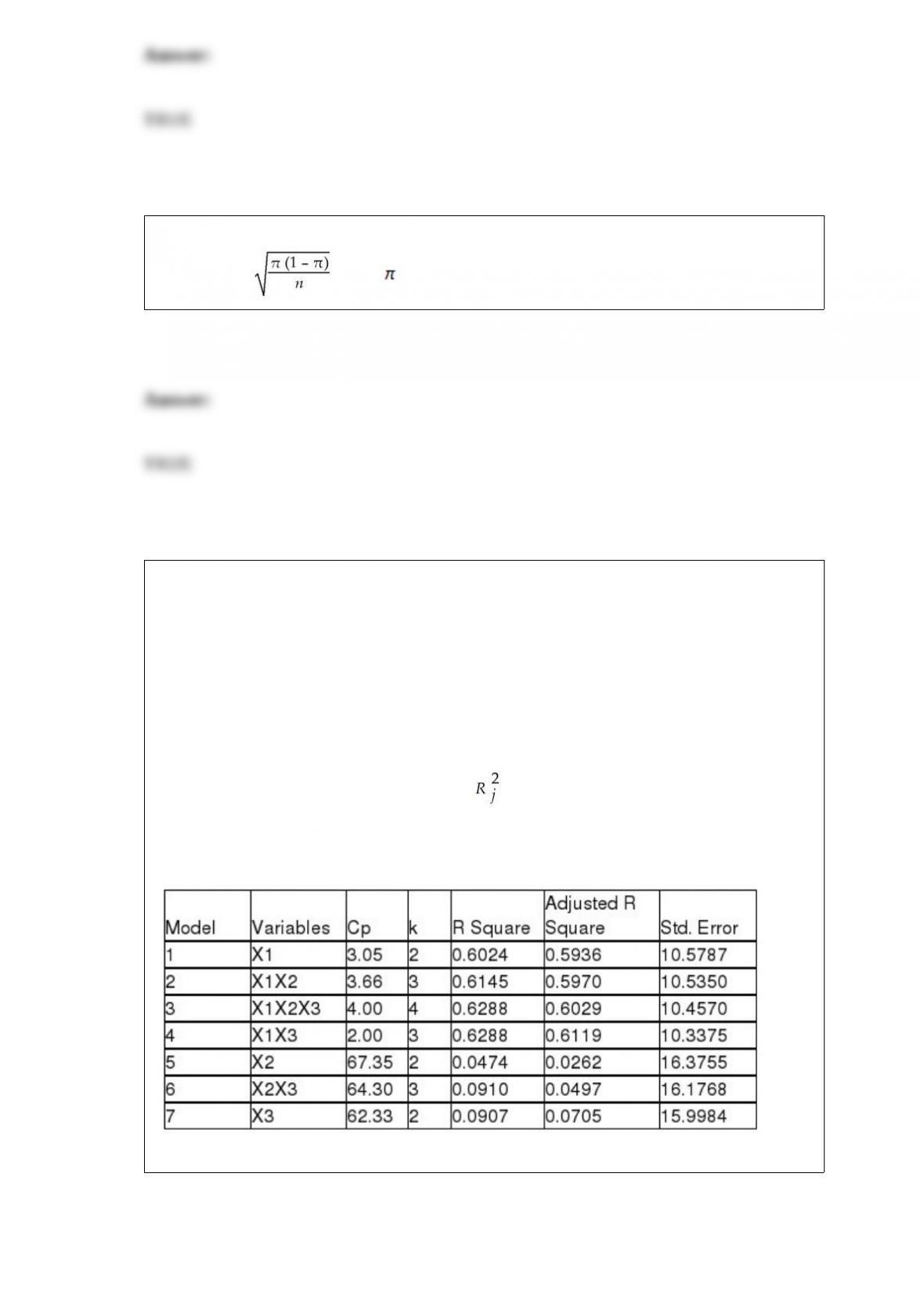
True or False: The standard deviation of the sampling distribution of a sample
proportion is where is the population proportion.
TABLE 15-4
The superintendent of a school district wanted to predict the percentage of students
passing a sixth-grade proficiency test. She obtained the data on percentage of students
passing the proficiency test (% Passing), daily mean of the percentage of students
attending class (% Attendance), mean teacher salary in dollars (Salaries), and
instructional spending per pupil in dollars (Spending) of 47 schools in the state.
Let Y = % Passing as the dependent variable, X1 = % Attendance, X2 = Salaries and X3
= Spending.
The coefficient of multiple determination ( ) of each of the 3 predictors with all the
other remaining predictors are, respectively, 0.0338, 0.4669, and 0.4743.
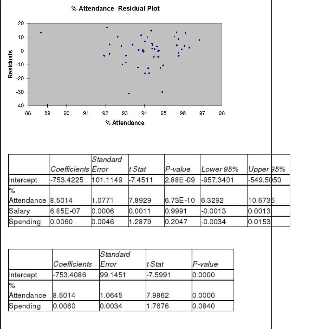
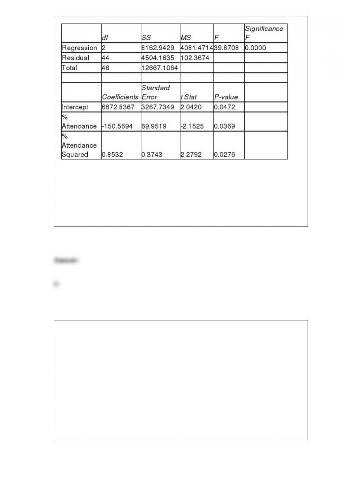
The output from the best-subset regressions is given below:
Following is the residual plot for % Attendance:

Following is the output of several multiple regression models:
Model (I):
Model (II):
Model (III):
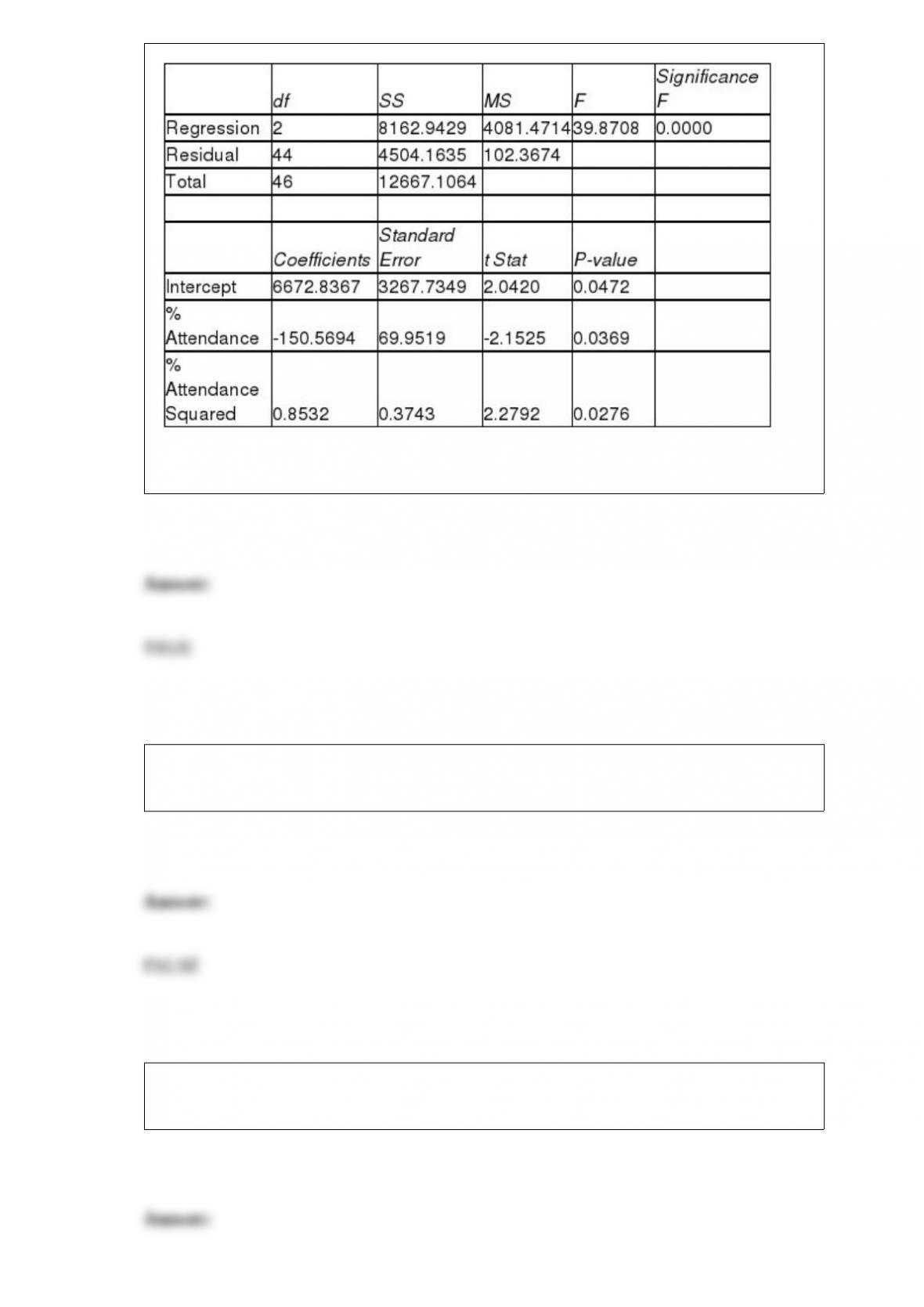
True or False: Referring to Table 15-4, the residual plot suggests that a nonlinear model
on % attendance may be a better model.
True or False: The number of customers arriving at a department store in a 5-minute
period has a binomial distribution.
True or False: The larger the Z score, the farther is the distance from the value to the
median.
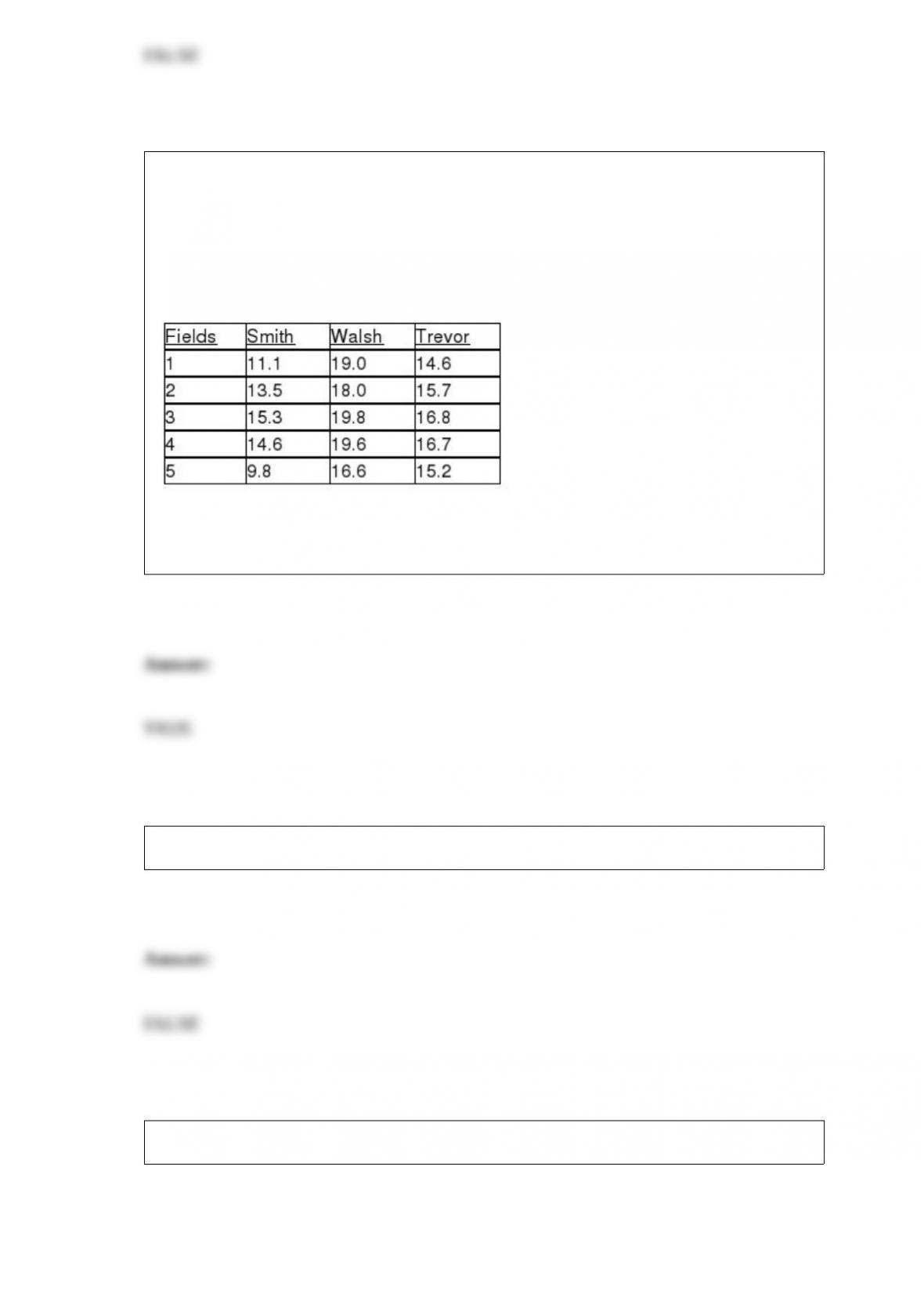
TABLE 11-10
An agronomist wants to compare the crop yield of 3 varieties of chickpea seeds. She
plants all 3 varieties of the seeds on each of 5 different patches of fields. She then
measures the crop yield in bushels per acre. Treating this as a randomized block design,
the results are presented in the table that follows.
True or False: Referring to Table 11-10, the randomized block F test is valid only if the
population of crop yields has the same variance for the 3 varieties.
True or False: There can be only one sample selected from a population.
True or False: Sampling error can be reduced by taking larger sample sizes.

True or False: The confidence interval estimate of the population mean is constructed
around the sample mean.
True or False: In real-world business analytics, filtering are typically performed on
large data based on complex conditional relationship.
TABLE 1-1
The manager of the customer service division of a major consumer electronics company
is interested in determining whether the customers who have purchased a Blu-ray
player made by the company over the past 12 months are satisfied with their products.
Referring to Table 1-1, the possible responses to the question “Are you happy,
indifferent, or unhappy with the performance per dollar spent on the Blu-ray player?”
result in
A) a nominal scale variable.
B) an ordinal scale variable.
C) an interval scale variable.
D) a ratio scale variable.
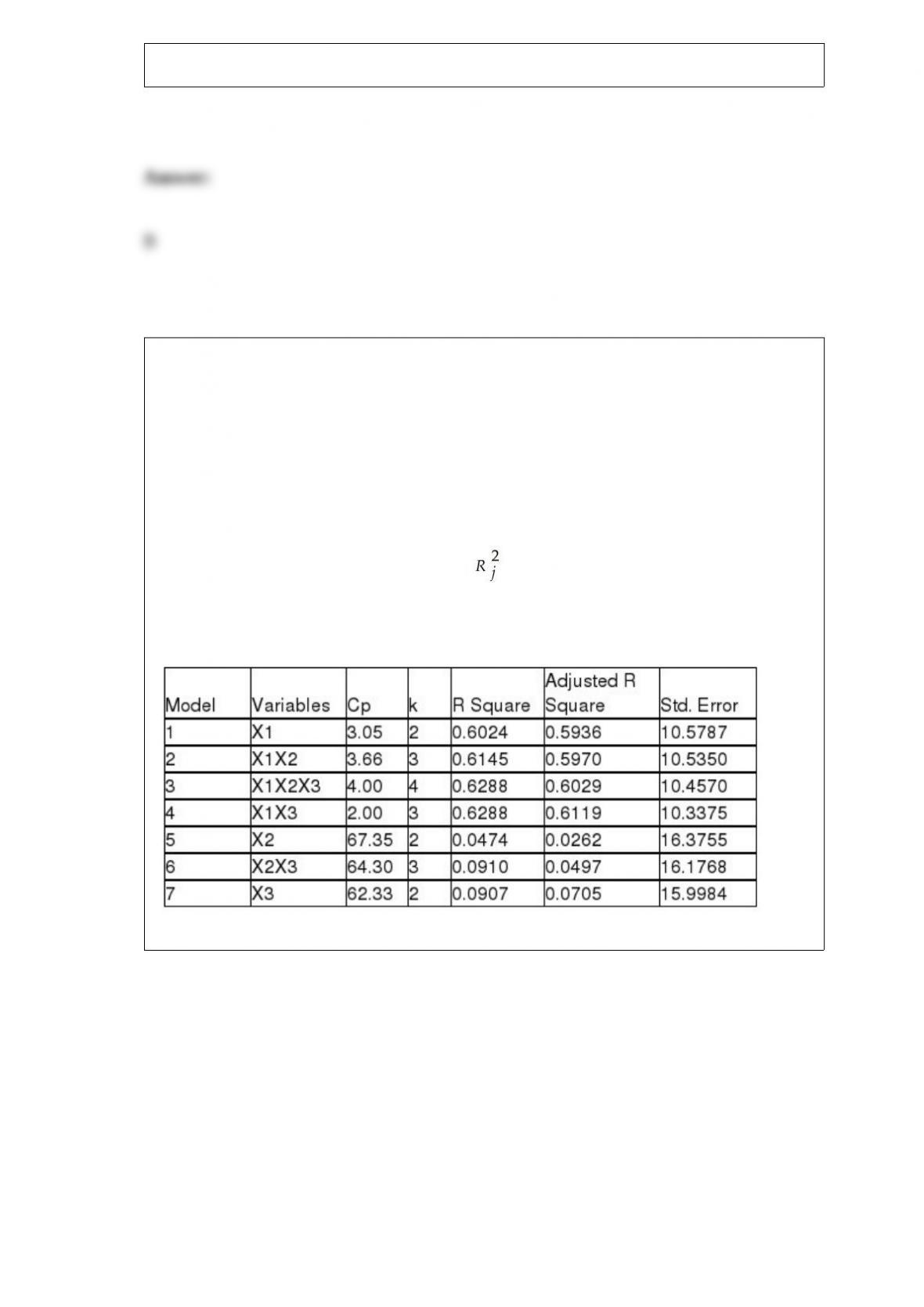
TABLE 15-4
The superintendent of a school district wanted to predict the percentage of students
passing a sixth-grade proficiency test. She obtained the data on percentage of students
passing the proficiency test (% Passing), daily mean of the percentage of students
attending class (% Attendance), mean teacher salary in dollars (Salaries), and
instructional spending per pupil in dollars (Spending) of 47 schools in the state.
Let Y = % Passing as the dependent variable, X1 = % Attendance, X2 = Salaries and X3
= Spending.
The coefficient of multiple determination ( ) of each of the 3 predictors with all the
other remaining predictors are, respectively, 0.0338, 0.4669, and 0.4743.
The output from the best-subset regressions is given below:
Following is the residual plot for % Attendance:
Following is the output of several multiple regression models:
Model (I):
Model (II):
Model (III):
Referring to Table 15-4, which of the following predictors should first be dropped to
remove collinearity?
A) X1
B) X2
C) X3
D) None of the above
TABLE 17-12
The marketing manager for a nationally franchised lawn service company would like to
study the characteristics that differentiate home owners who do and do not have a lawn
service. A random sample of 30 home owners located in a suburban area near a large
city was selected; 15 did not have a lawn service (code 0) and 15 had a lawn service
(code 1). Additional information available concerning these 30 home owners includes
family income (Income, in thousands of dollars), lawn size (Lawn Size, in thousands of
square feet), attitude toward outdoor recreational activities (Attitude 0 = unfavorable, 1
= favorable), number of teenagers in the household (Teenager), and age of the head of
the household (Age).
The Minitab output is given below:
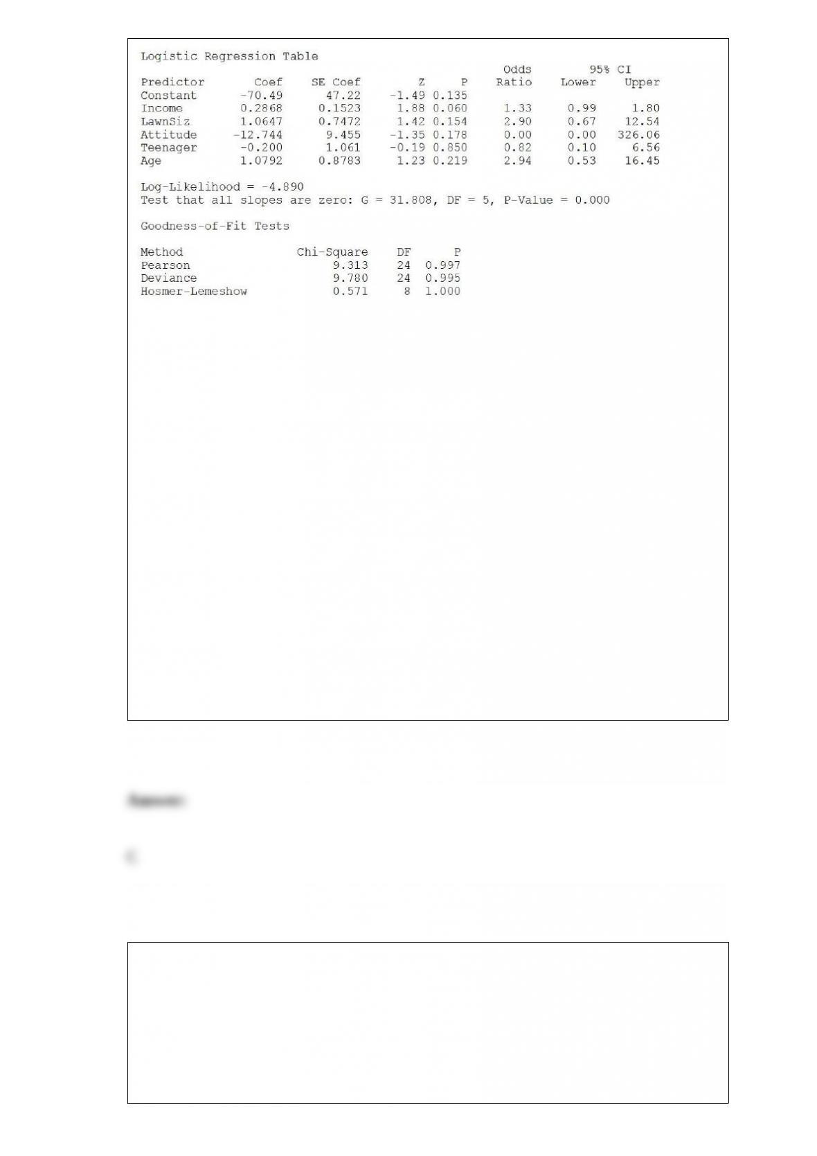
Referring to Table 17-12, which of the following is the correct interpretation for the
Attitude slope coefficient?
A) Holding constant the effect of the other variables, the estimated number of lawn
services purchased is 12.74 lower for a home owner who has a favorable attitude
toward outdoor recreational activities than one that has an unfavorable attitude.
B) Holding constant the effect of the other variables, the estimated odds ratio of
purchasing a lawn service is 12.74 lower for a home owner who has a favorable attitude
toward outdoor recreational activities than one that has an unfavorable attitude.
C) Holding constant the effect of the other variables, the estimated natural logarithm of
the odds ratio of purchasing a lawn service is 12.74 lower for a home owner who has a
favorable attitude toward outdoor recreational activities than one that has an
unfavorable attitude.
D) Holding constant the effect of the other variables, the estimated probability of
purchasing a lawn service is 12.74 lower for a home owner who has a favorable attitude
toward outdoor recreational activities than one that has an unfavorable attitude.
What do we mean when we say that a simple linear regression model is ‘statistically”
useful?
A) All the statistics computed from the sample make sense.
B) The model is an excellent predictor of Y.

C) The model is “practically” useful for predicting Y.
D) The model is a better predictor of Y than the sample mean, .
Referring to Table 14-18, which of the following is the correct
interpretation for the SAT slope coecient?
TABLE 14-18
A logistic regression model was estimated in order to predict the
probability that a randomly chosen university or college would be a
private university using information on mean total Scholastic Aptitude
Test score (SAT) at the university or college and whether the TOEFL
criterion is at least 90 (Toe90 = 1 if yes, 0 otherwise). The
dependent variable, Y, is school type (Type = 1 if private and 0
otherwise).
The PHStat output is given below:
A) Holding constant the effect of Toe90, the estimated mean value
of school type increases by 0.0028 for each increase of one point in
average SAT score.
B) Holding constant the effect of Toe90, the estimated school type
increases by 0.0028 for each increase of one point in average SAT
score.
C) Holding constant the effect of Toe90, the estimated probability of
the school being a private school increases by 0.0028 for each
increase of one point in mean SAT score.
D) Holding constant the effect of Toe90, the estimated natural
logarithm of the odds ratio of the school being a private school
increases by 0.0028 for each increase of one point in mean SAT
score.

In a perfectly symmetrical distribution,
A) the range equals the interquartile range.
B) the interquartile range equals the arithmetic mean.
C) the median equals the arithmetic mean.
D) the variance equals the standard deviation.
TABLE 11-8
A physician and president of a Tampa Health Maintenance Organization (HMO) are
attempting to show the benefits of managed health care to an insurance company. The
physician believes that certain types of doctors are more cost-effective than others. One
theory is that Primary Specialty is an important factor in measuring the
cost-effectiveness of physicians. To investigate this, the president obtained independent
random samples of 20 HMO physicians from each of 4 primary specialties – General
Practice (GP), Internal Medicine (IM), Pediatrics (PED), and Family Physicians (FP) –
and recorded the total charges per member per month for each. A second factor which
the president believes influences total charges per member per month is whether the
doctor is a foreign or USA medical school graduate. The president theorizes that foreign
graduates will have higher mean charges than USA graduates. To investigate this, the
president also collected data on 20 foreign medical school graduates in each of the 4
primary specialty types described above. So information on charges for 40 doctors (20
foreign and 20 USA medical school graduates) was obtained for each of the 4
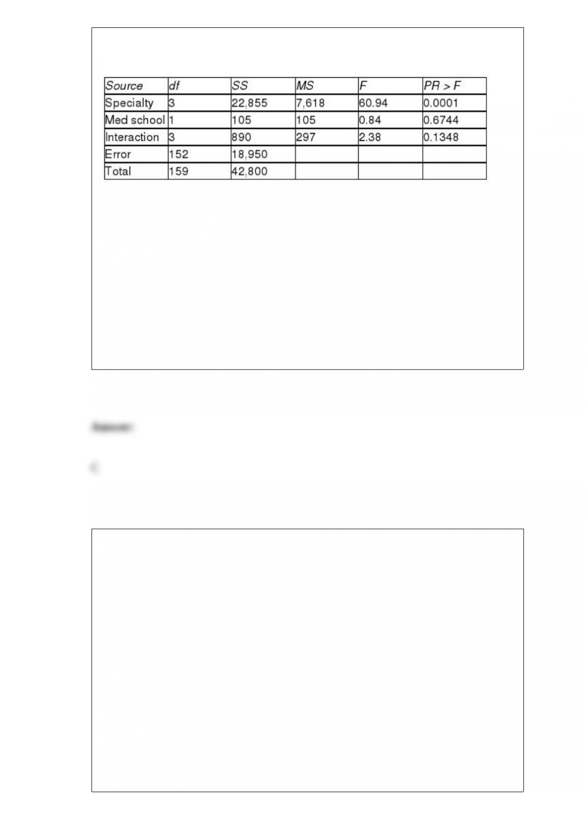
specialties. The results for the ANOVA are summarized in the following table.
Referring to Table 11-8, what degrees of freedom should be used to determine the
critical value of the F ratio against which to test for differences between the mean
charges of foreign and USA medical school graduates?
A) numerator df = 1, denominator df = 159
B) numerator df = 3, denominator df = 159
C) numerator df = 1, denominator df = 152
D) numerator df = 3, denominator df = 152
What type of probability distribution will most likely be used to analyze warranty repair
needs on new cars in the following problem?
The service manager for a new automobile dealership reviewed dealership records of
the past 20 sales of new cars to determine the number of warranty repairs he will be
called on to perform in the next 90 days. Corporate reports indicate that the probability
any one of their new cars needs a warranty repair in the first 90 days is 0.05. The
manager assumes that calls for warranty repair are independent of one another and is
interested in predicting the number of warranty repairs he will be called on to perform
in the next 90 days for this batch of 20 new cars sold.
A) Binomial distribution
B) Poisson distribution
C) Hypergeometric distribution

D) None of the above
The Dean of Students mailed a survey to a total of 400 students. The sample included
100 students randomly selected from each of the freshman, sophomore, junior, and
senior classes on campus last term. What sampling method was used?
A) simple random sample
B) systematic sample
C) stratified sample
D) cluster sample
Referring to Table 14-5, what are the predicted sales (in millions of dollars) for a
company spending $100 million on capital and $100 million on wages?
TABLE 14-5
A microeconomist wants to determine how corporate sales are influenced by capital and
wage spending by companies. She proceeds to randomly select 26 large corporations
and record information in millions of dollars. The Microsoft Excel output below shows
results of this multiple regression.
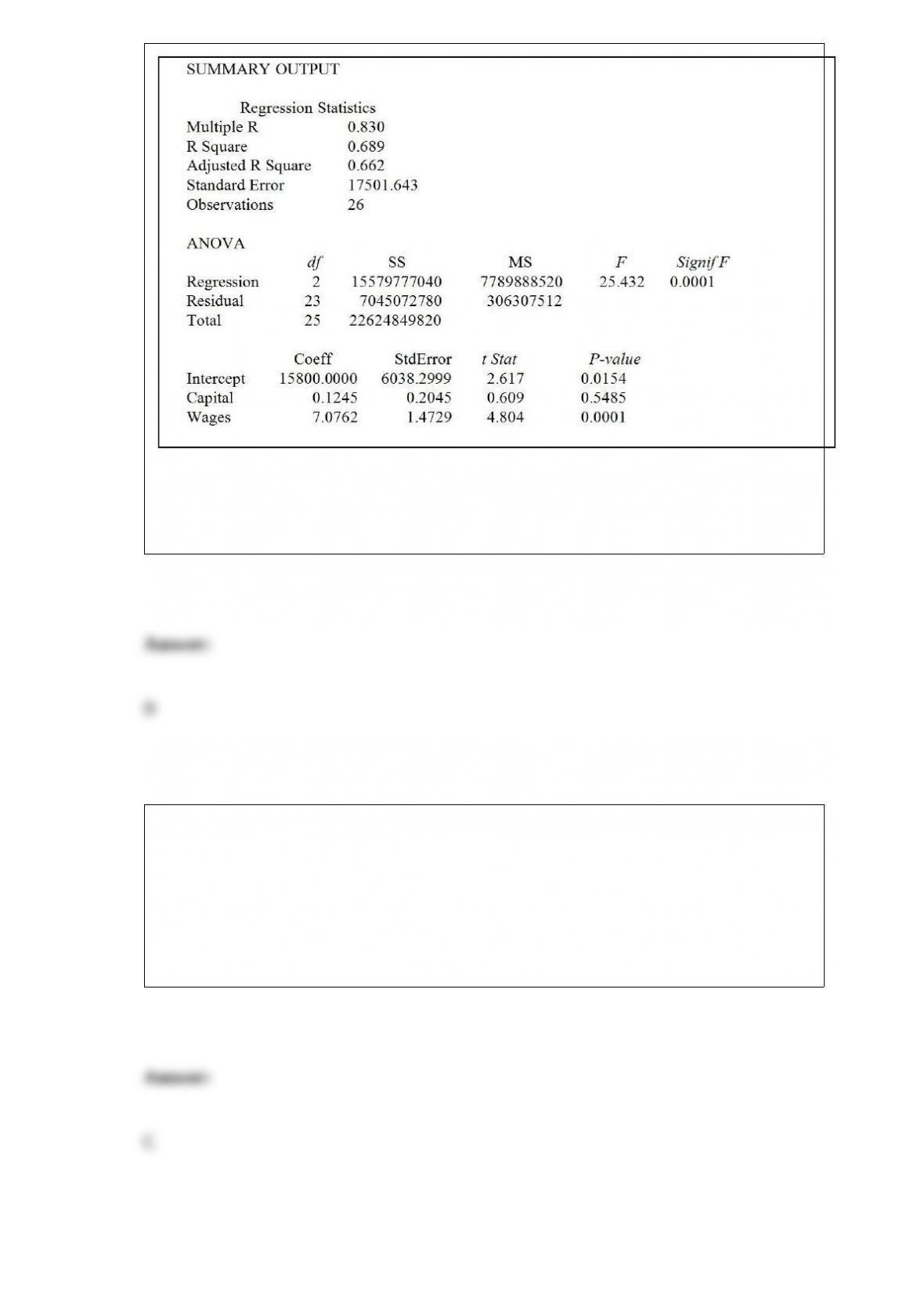
A) 15,800.00
B) 16,520.07
C) 17,277.49
D) 20,455.98
Data on the amount of money made in a year by 1,000 families in a small town were
collected. You want to know the difference in the amount of money made in that year
by the middle 50% of the 1,000 families. Which of the following would you compute?
A) Arithmetic mean
B) Median
C) Interquartile range
D) Coefficient of correlation

In a contingency table, the number of rows and columns
A) must always be the same.
B) must always be 2.
C) must add to 100%.
D) None of the above.
According to a survey of American households, the probability that the residents own 2
cars if annual household income is over $50,000 is 80%. Of the households surveyed,
60% had incomes over $50,000 and 70% had 2 cars. The probability that annual
household income is over $50,000 if the residents of a household do not own 2 cars is
A) 0.12.
B) 0.18.
C) 0.40.
D) 0.70.
TABLE 12-9
Many companies use well-known celebrities as spokespersons in their TV
advertisements. A study was conducted to determine whether brand awareness of
female TV viewers and the gender of the spokesperson are independent. Each in a
sample of 300 female TV viewers was asked to identify a product advertised by a
celebrity spokesperson. The gender of the spokesperson and whether or not the viewer
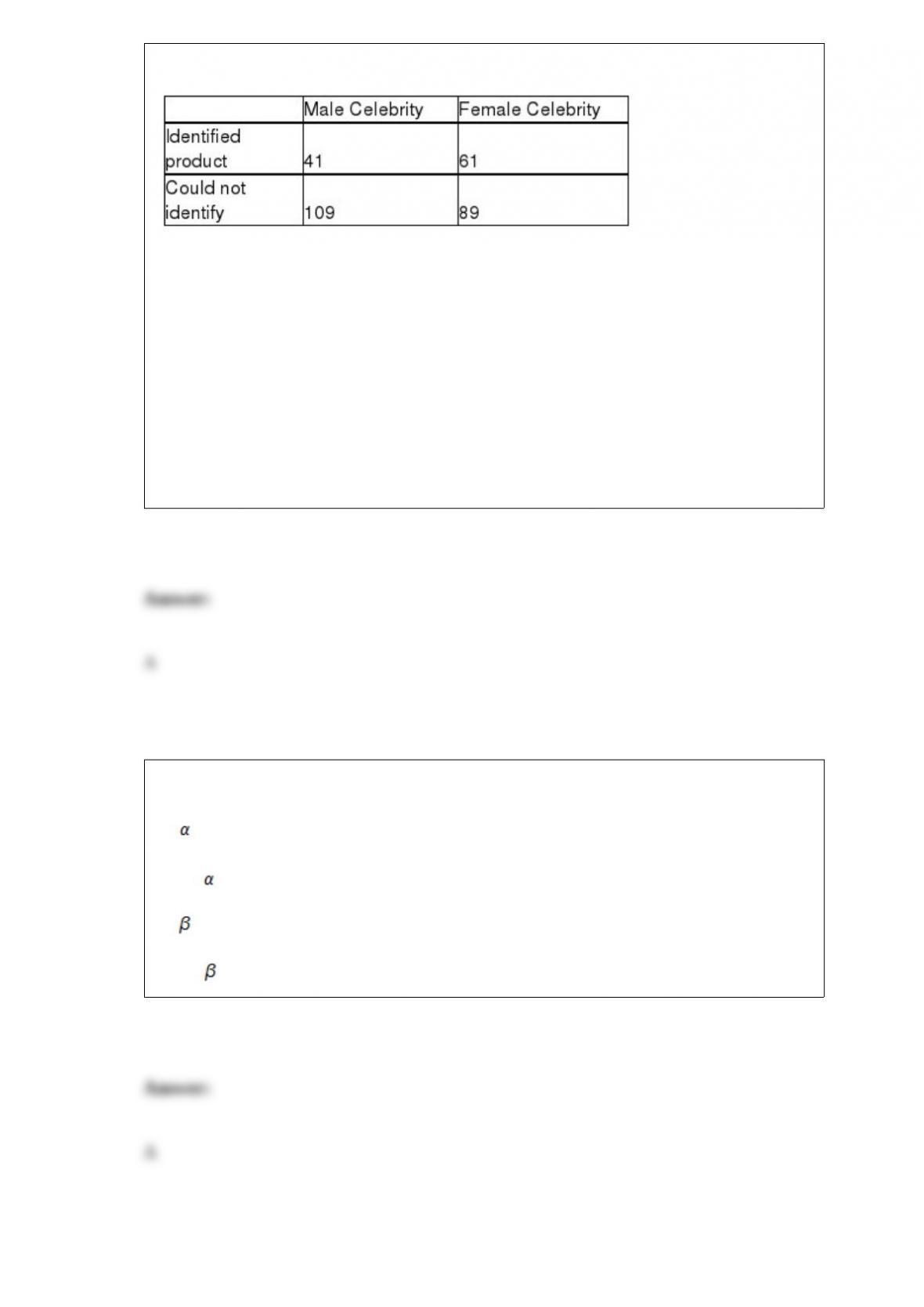
could identify the product was recorded. The numbers in each category are given below.
Referring to Table 12-9, which test would be used to properly analyze the data in this
experiment?
A) X2 test for independence
B) X2 test for differences among more than two proportions
C) Wilcoxon rank sum test for independent populations
D) Kruskal-Wallis rank test
The symbol for the probability of committing a Type I error of a statistical test is
A) .
B) 1 – .
C) .
D) 1 – .

Which of the following statements is not true about the level of significance in a
hypothesis test?
A) The larger the level of significance, the more likely you are to reject the null
hypothesis.
B) The level of significance is the maximum risk we are willing to accept in making a
Type I error.
C) The significance level is also called the level.
D) The significance level is another name for Type II error.
A certain type of rare gem serves as a status symbol for many of its owners. In theory,
for low prices, the demand increases and it decreases as the price of the gem increases.
However, experts hypothesize that when the gem is valued at very high prices, the
demand increases with price due to the status owners believe they gain in obtaining the
gem. Data on price and quantity sold were collected for a sample of 35 rare gems of this
type. Which of the following would be the most appropriate analysis to perform?
A) Quadratic regression model
B) Exponential smoothing
C) Autoregressive modeling for trend fitting and forecasting
D) Least-squares forecasting with monthly or quarterly data
TABLE 15-3
A chemist employed by a pharmaceutical firm has developed a muscle relaxant. She
took a sample of 14 people suffering from extreme muscle constriction. She gave each a
vial containing a dose (X) of the drug and recorded the time to relief (Y) measured in
seconds for each. She fit a curvilinear model to this data. The results obtained by
Microsoft Excel follow
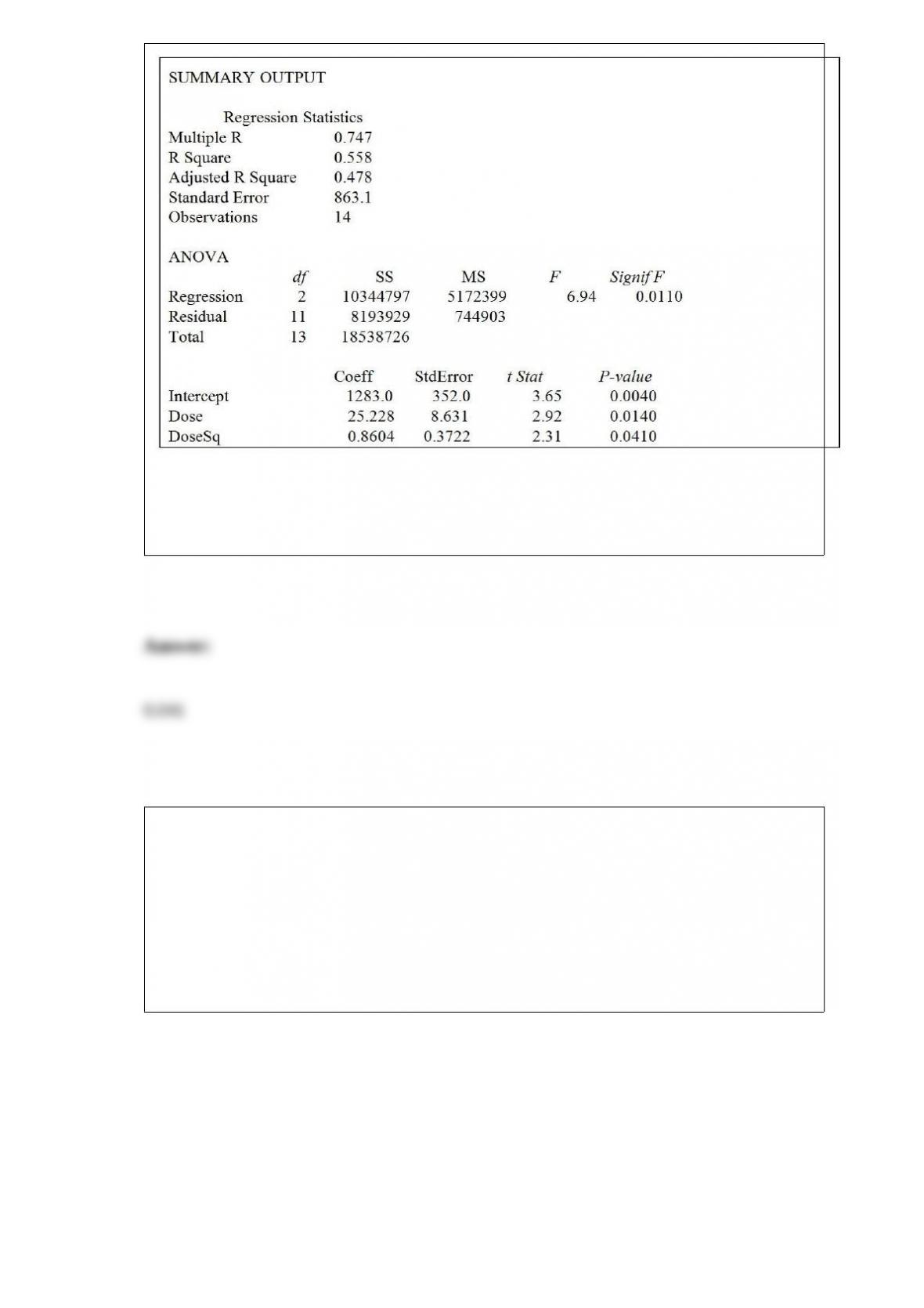
Referring to Table 15-3, suppose the chemist decides to use a t test to determine if there
is a significant difference between a linear model and a curvilinear model that includes
a linear term. The p-value of the test statistic for the contribution of the curvilinear term
is ________.
TABLE 17-11
A logistic regression model was estimated in order to predict the probability that a
randomly chosen university or college would be a private university using information
on mean total Scholastic Aptitude Test score (SAT) at the university or college, the
room and board expense measured in thousands of dollars (Room/Brd), and whether the
TOEFL criterion is at least 550 (Toefl550 = 1 if yes, 0 otherwise.) The dependent
variable, Y, is school type (Type = 1 if private and 0 otherwise).
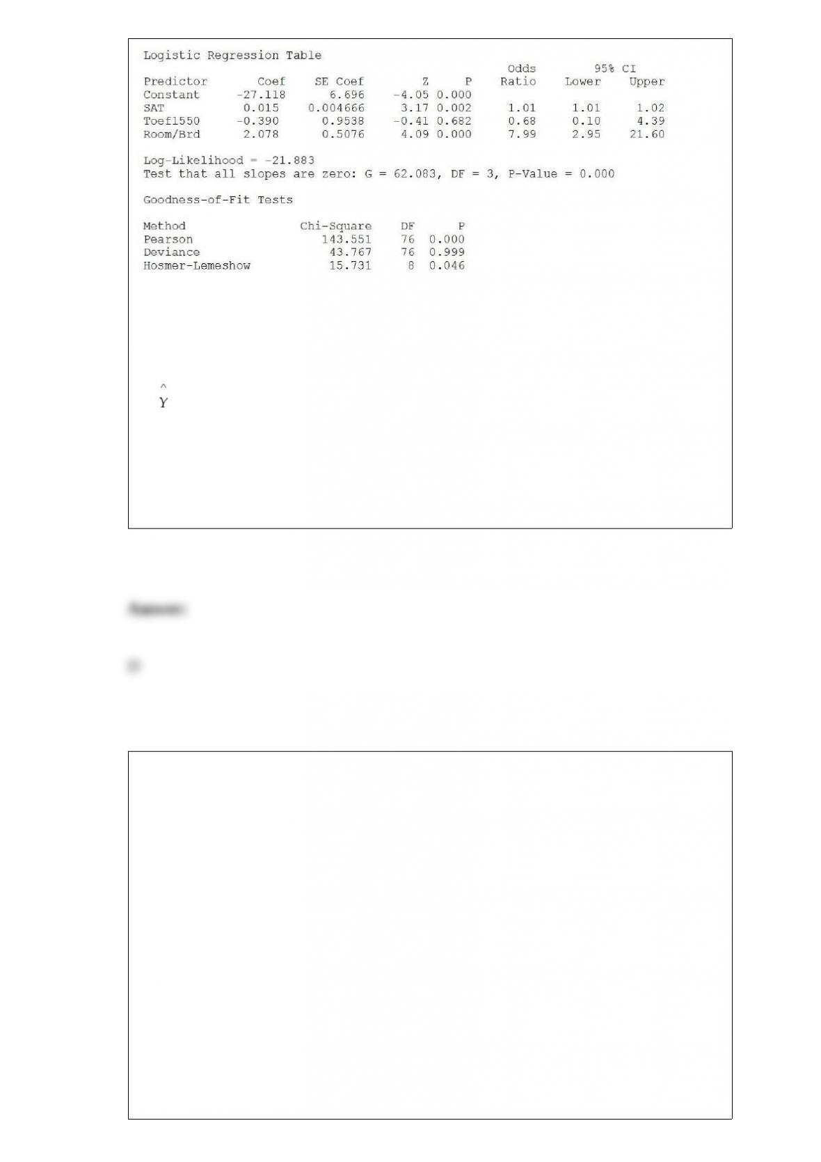
Referring to Table 17-11, which of the following is the correct expression for the
estimated model?
A)Y= -27.118 + 0.015SAT– 0.390Toefl550 + 2.078Room / Brd
B) = -27.118 + 0.015 SAT – 0.390 Toefl550 + 2.078 Room / Brd
C) ln (odds ratio) = -27.118 + 0.015 SAT – 0.390 Toefl550 + 2.078 Room / Brd
D) ln (estimated odds ratio) = -27.118 + 0.015 SAT – 0.390 Toefl550 + 2.078 Room /
Brd
TABLE 9-9
The president of a university claimed that the entering class this year appeared to be
larger than the entering class from previous years but their mean SAT score is lower
than previous years. He took a sample of 20 of this year’s entering students and found
that their mean SAT score is 1,501 with a standard deviation of 53. The university’s
record indicates that the mean SAT score for entering students from previous years is
1,520. He wants to find out if his claim is supported by the evidence at a 5% level of
significance.
Referring to Table 9-9, which of the following best describes the Type II error?
A) The president concludes that the mean SAT score of the entering students is lower
than previous years when it is indeed not lower.
B) The president concludes that the mean SAT score of the entering students is higher
than previous years when it is indeed not higher.
C) The president concludes that the mean SAT score of the entering students is not
lower than previous years when it is indeed lower.
D) The president concludes that the mean SAT score of the entering students is not
higher than previous years when it is indeed higher.
Referring to Table 17-10 and using both Model 1 and Model 2, what is the value of the
test statistic for testing whether the independent variables that are not significant
individually are also not significant as a group in explaining the variation in the
dependent variable at a 5% level of significance?
TABLE 9-3
An appliance manufacturer claims to have developed a compact microwave oven that
consumes a mean of no more than 250 W. From previous studies, it is believed that
power consumption for microwave ovens is normally distributed with a population
standard deviation of 15 W. A consumer group has decided to try to discover if the
claim appears true. They take a sample of 20 microwave ovens and find that they
consume a mean of 257.3 W.
Referring to Table 9-3, for a test with a level of significance of 0.05, the critical value
would be ________.
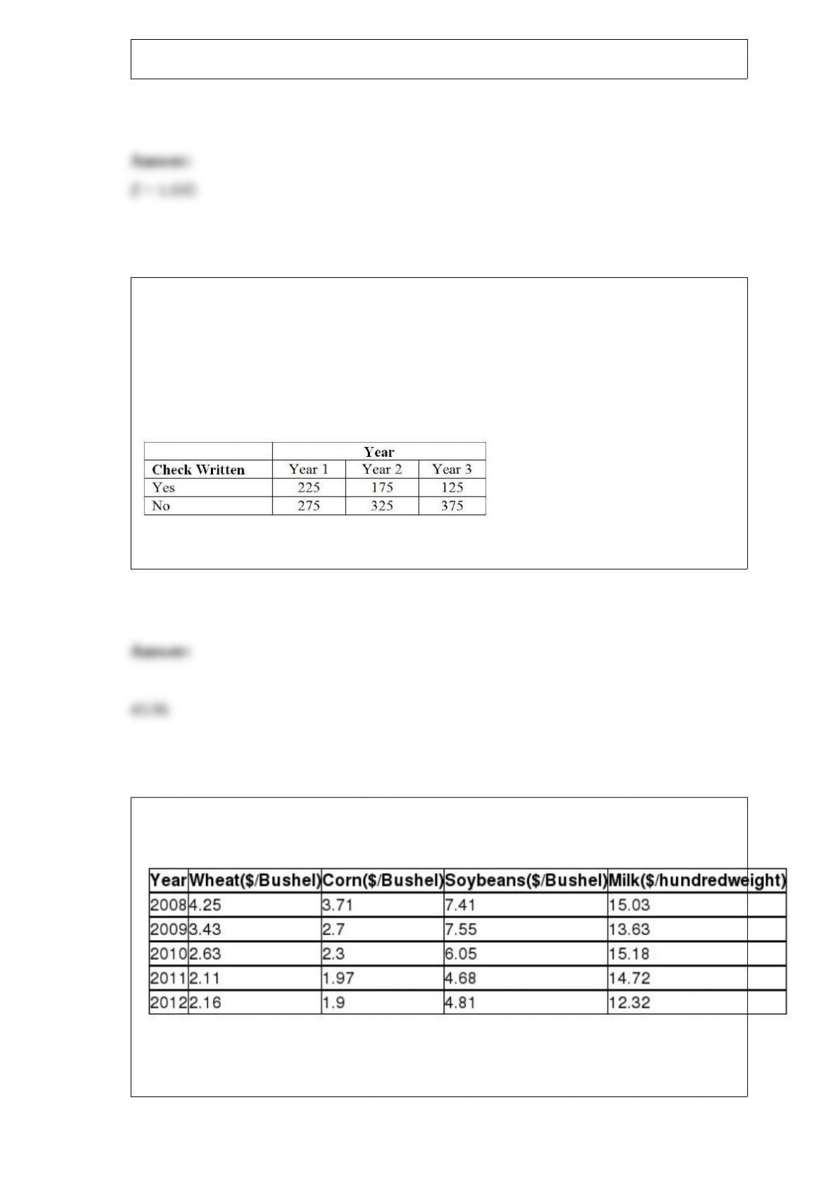
TABLE 12-6
According to an article in Marketing News, fewer checks are being written at the
grocery store checkout than in the past. To determine whether there is a difference in
the proportion of shoppers who pay by check among three consecutive years at a 0.05
level of significance, the results of a survey of 500 shoppers in three consecutive years
are obtained and presented below.
Referring to Table 12-6, what is the value of the test statistic?
TABLE 16-16
Given below are the prices of a basket of four food items from 2008 to 2012.
Referring to Table 16-16, what is the Paasche price index for the basket of four food
items in 2011 that consisted of 60 bushels of wheat, 40 bushels of corn, 35 bushels of
soybeans and 70 hundredweight of milk in 2011 using 2008 as the base year?
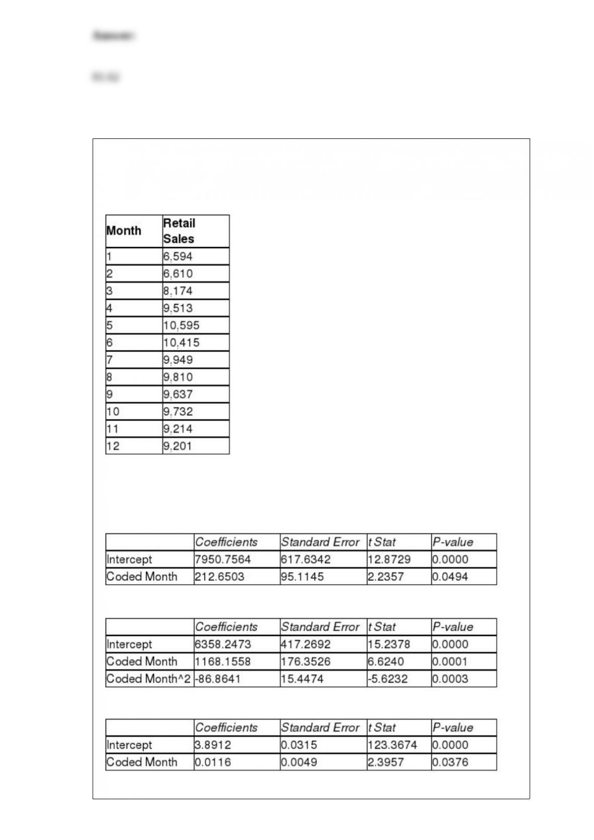
TABLE 16-13
Given below is the monthly time-series data for U.S. retail sales of building materials
over a specific year.
The results of the linear trend, quadratic trend, exponential trend, first-order
autoregressive, second-order autoregressive and third-order autoregressive model are
presented below in which the coded month for the 1st month is 0:
Linear trend model:
Quadratic trend model:
Exponential trend model:
First-order autoregressive:
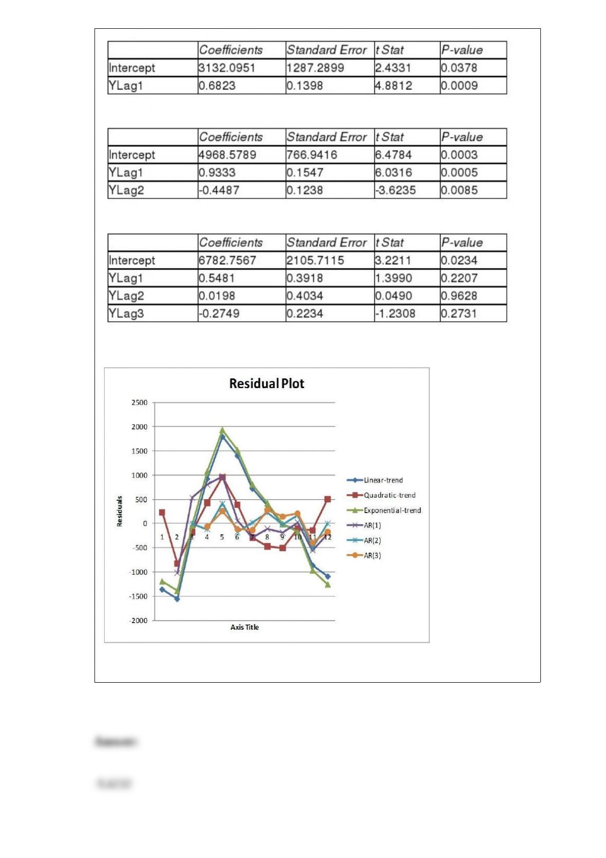
Second-order autoregressive:
Third-order autoregressive:
Below is the residual plot of the various models:
Referring to Table 16-13, what is the value of the t test statistic for testing the
significance of the quadratic term in the quadratic-trend model?
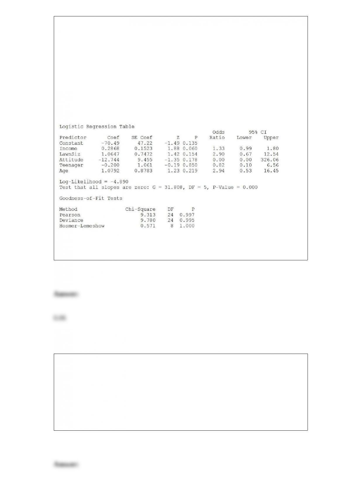
TABLE 17-12
The marketing manager for a nationally franchised lawn service company would like to
study the characteristics that differentiate home owners who do and do not have a lawn
service. A random sample of 30 home owners located in a suburban area near a large
city was selected; 15 did not have a lawn service (code 0) and 15 had a lawn service
(code 1). Additional information available concerning these 30 home owners includes
family income (Income, in thousands of dollars), lawn size (Lawn Size, in thousands of
square feet), attitude toward outdoor recreational activities (Attitude 0 = unfavorable, 1
= favorable), number of teenagers in the household (Teenager), and age of the head of
the household (Age).
The Minitab output is given below:
Referring to Table 17-12, what is the p-value of the test statistic when testing whether
Income makes a significant contribution to the model in the presence of the other
independent variables?
TABLE 7-2
The mean selling price of new homes in a small town over a year was $115,000. The
population standard deviation was $25,000. A random sample of 100 new home sales
from this city was taken.
Referring to Table 7-2, what is the probability that the sample mean selling price was
between $113,000 and $117,000?