Chapter 13 – Multiple Regression
x2
0.9210
0.190
x3
-0.510
0.920
a.
Compute the coefficient of determination.
b.
Perform a t test and determine whether or not the coefficient of the variable “level of
education” (i.e., x2) is significantly different from zero. Let α = 0.05.
c.
At α = 0.05, perform an F test and determine whether or not the regression model is significant.
d.
As you note the coefficient of x3 is -0.510. Fully interpret the meaning of this coefficient.
a.
0.4286
b.
c.
d.
Male’s income is lower than female’s by $510
88. A multiple regression analysis between yearly income (y in $1,000s), college grade point average (x1), age of the
individuals (x2), and the gender of the individual (x3; zero representing female and one representing male) was performed
on a sample of 10 people, and the following results were obtained using Excel.
ANOVA
df
SS
MS
F
Regression
360.59
Residual
23.91
Coefficients
Standard Error
Intercept
4.0928
1.4400
x1
10.0230
1.6512
x2
0.1020
0.1225
x3
-4.4811
1.4400
a.
Write the regression equation for the above.
b.
Interpret the meaning of the coefficient of x3.
c.
Compute the coefficient of determination.
d.
Is the coefficient of x1 significant? Use α = 0.05.
e.
Is the coefficient of x2 significant? Use α = 0.05.
f.
Is the coefficient of x3 significant? Use α = 0.05.
g.
Perform an F test and determine whether or not the model is significant.
a.
thousands).
c.
0.9378
d.
e.
g.
89. The following results were obtained from a multiple regression analysis.
Chapter 13 – Multiple Regression
Source of Variation
Degrees of
Freedom
Sum of
Squares
Mean
Square
F
Regression
900
Error
35
Total
39
4,980
a.
How many independent variables were involved in this model?
b.
How many observations were involved?
c.
Determine the F statistic.
a.
b.
40
c.
1.93
90. Shown below is a partial Excel output from a regression analysis.
ANOVA
df
SS
MS
F
Regression
60
Residual
Total
19
140
Coefficients
Standard Error
Intercept
10.00
2.00
x1
-2.00
1.50
x2
6.00
2.00
x3
-4.00
1.00
a.
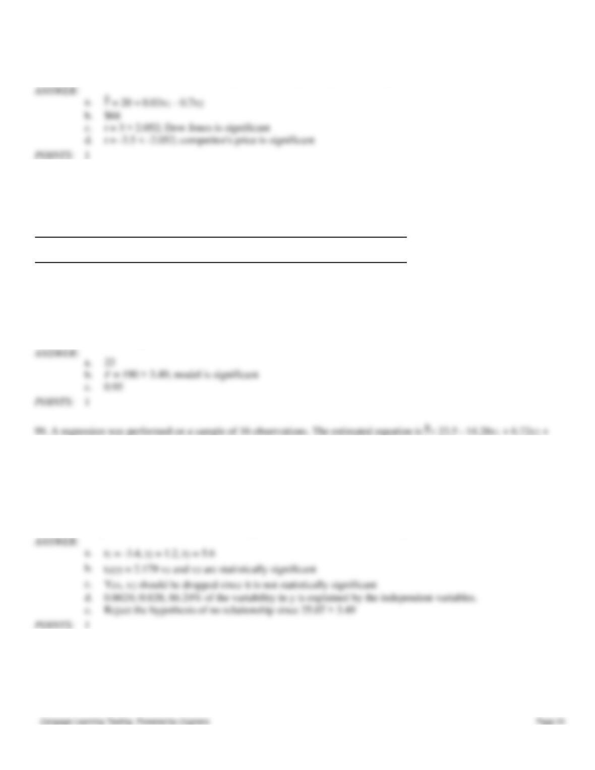
Use the above results and write the regression equation.
b.
Compute the coefficient of determination and fully interpret its meaning.
c.
Is the regression model significant? Perform an F test and let α = 0.05.
d.
At α = 0.05, test to see if there is a relation between x1 and y.
e.
At α = 0.05, test to see if there is a relation between x3 and y.
a.
independent variables.
c.
d.
e.
91. In order to determine whether or not the sales volume of a company (y in millions of dollars) is related to advertising
expenditures (x1 in millions of dollars) and the number of salespeople (x2), data were gathered for 10 years. Part of the
Excel output is shown below.
ANOVA
df
SS
MS
F
Regression
321.11
Residual
63.39
Chapter 13 – Multiple Regression
Coefficients
Standard Error
Intercept
7.0174
1.8972
x1
8.6233
2.3968
x2
0.0858
0.1845
a.
Use the above results and write the regression equation that can be used to predict sales.
b.
Estimate the sales volume for an advertising expenditure of 3.5 million dollars and 45
salespeople. Give your answer in dollars.
c.
At α = 0.01, test to determine if the fitted equation developed in Part a represents a significant
relationship between the independent variables and the dependent variable.
d.
At α = 0.05, test to see if β1 is significantly different from zero.
e.
Determine the multiple coefficient of determination.
f.
Compute the adjusted coefficient of determination.
a.
$41,059,950
c.
e.
0.8351
f.
0.7879
92. In order to determine whether or not the number of automobiles sold per day (y) is related to price (x1 in $1,000), and
the number of advertising spots (x2), data were gathered for 7 days. Part of the Excel output is shown below.
ANOVA
df
SS
MS
F
Regression
40.700
Residual
1.016
Coefficients
Standard Error
Intercept
0.8051
x1
0.4977
0.4617
x2
0.4733
0.0387
a.
Determine the least squares regression function relating y to x1 and x2.
b.
If the company charges $20,000 for each car and uses 10 advertising spots, how many cars
would you expect them to sell in a day?
c.
At α = 0.05, test to determine if the fitted equation developed in Part a represents a significant
relationship between the independent variables and the dependent variable.
d.
At α = 0.05, test to see if β1 is significantly different from zero.
e.
Determine the multiple coefficient of determination.
a.
c.
t = 1.078 < 2.776; not significant
93. The following is part of the results of a regression analysis involving sales (y in millions of dollars), advertising
expenditures (x1 in thousands of dollars), and number of salespeople (x2) for a corporation. The regression was performed
on a sample of 10 observations.
Coefficient
Standard Error
Constant
-11.340
20.412
x1
0.798
0.332
x2
0.141
0.278
a.
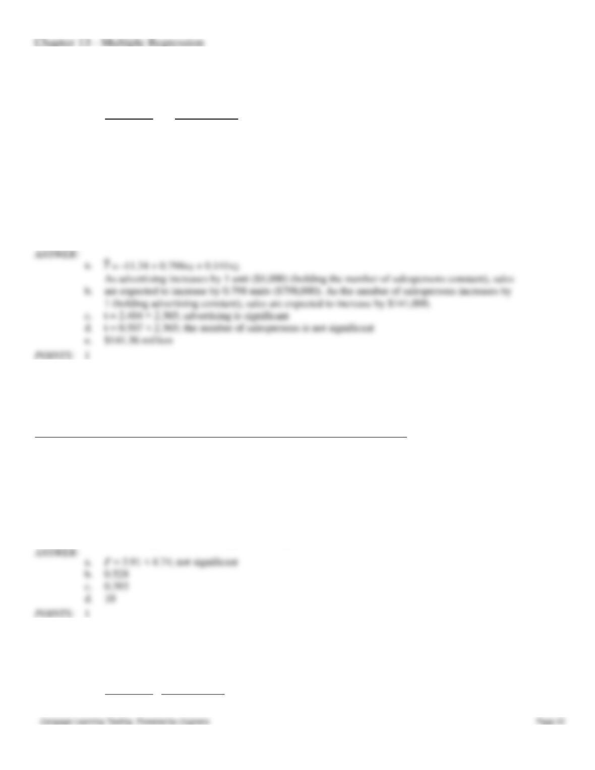
Write the regression equation.
b.
Interpret the coefficients of the estimated regression equation found in Part (a).
c.
At α =0.05, test for the significance of the coefficient of advertising.
d.
At α =0.05, test for the significance of the coefficient of number of salespeople.
e.
If the company uses $50,000 in advertisement and has 800 salespersons, what are the expected
sales? Give your answer in dollars.
As advertising increases by 1 unit ($1,000) (holding the number of salespersons constant), sales
c.
t = 2.404 > 2.365; advertising is significant
d.
t = 0.507 < 2.365; the number of salespersons is not significant
e.
$141.36 million
1
94. The following is part of the results of a regression analysis involving sales (y in millions of dollars), advertising
expenditures (x1 in thousands of dollars), and number of sales people (x2) for a corporation:
Source of Variation
Degrees of
Freedom
Sum of
Squares
Mean
Square
F
Regression
2
822.088
Error
7
736.012
a.
At α = 0.05 level of significance, test to determine if the model is significant. That is,
determine if there exists a significant relationship between the independent variables and the
dependent variable.
b.
Determine the multiple coefficient of determination.
c.
Determine the adjusted multiple coefficient of determination.
d.
What has been the sample size for this regression analysis?
a.
b.
0.528
c.
0.393
d.
10
1
95. Below you are given a partial Excel output based on a sample of 12 observations relating the number of personal
computers sold by a computer shop per month (y), unit price (x1 in $1,000) and the number of advertising spots (x2) used
on a local television station.
Coefficient
Standard Error
Intercept
17.145
7.865
x1
-0.104
3.282
x2
1.376
0.250
a.
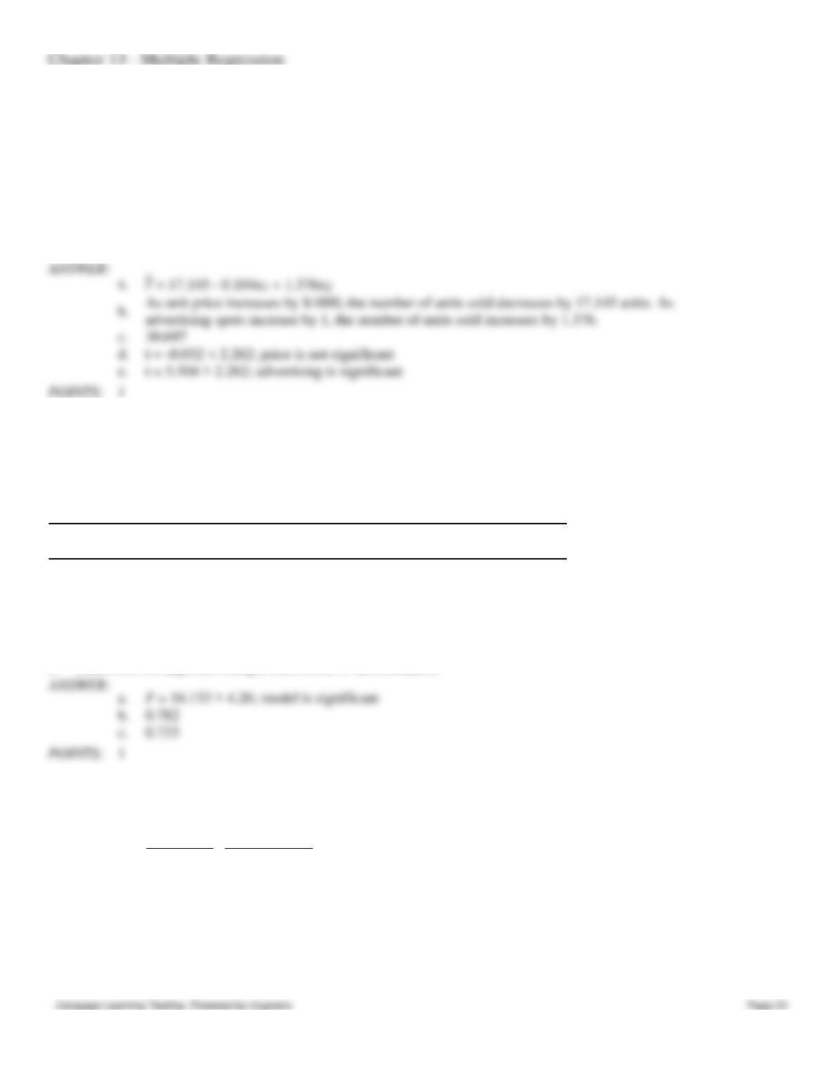
Use the output shown above and write an equation that can be used to predict the monthly sales
of computers.
b.
Interpret the coefficients of the estimated regression equation found in Part a.
c.
If the company charges $2,000 for each computer and uses 10 advertising spots, how many
computers would you expect them to sell?
d.
At α = 0.05, test to determine if the price is a significant variable.
e.
At α = 0.05, test to determine if the number of advertising spots is a significant variable.
advertising spots increase by 1, the number of units sold increases by 1.376.
c.
30.697
d.
t = -0.032 < 2.262; price is not significant
e.
t = 5.504 > 2.262; advertising is significant
1
96. Below you are given a partial ANOVA table based on a sample of 12 observations relating the number of personal
computers sold by a computer shop per month (y), unit price (x1 in $1,000) and the number of advertising spots (x2) they
used on a local television station.
Source of Variation
Degrees of
Freedom
Sum of
Squares
Mean
Square
F
Regression
2
655.955
Error
9
Total
838.917
a.
At α = 0.05 level of significance, test to determine if the model is significant. That is,
determine if there exists a significant relationship between the independent variables and the
dependent variable.
b.
Determine the multiple coefficient of determination.
c.
Determine the adjusted multiple coefficient of determination.
a.
b.
0.782
c.
0.733
1
97. Below you are given a partial Excel output based on a sample of 30 days of the price of a company’s stock (y in
dollars), the Dow Jones industrial average (x1), and the stock price of the company’s major competitor (x2 in dollars).
Coefficient
Standard Error
Intercept
20.000
5.455
x1
0.030
0.010
x2
-0.70
0.200
a.
Use the output shown above and write an equation that can be used to predict the price of the
stock.
b.
If the Dow Jones Industrial Average is 2650 and the price of the competitor is $45, what would
you expect the price of the stock to be?
Chapter 13 – Multiple Regression
c.
At α = 0.05, test to determine if the Dow Jones average is a significant variable.
d.
At α = 0.05, test to determine if the stock price of the major competitor is a significant variable.
b.
$68
c.
d.
98. Below you are given a partial ANOVA table relating the price of a company’s stock (y in dollars), the Dow Jones
industrial average (x1), and the stock price of the company’s major competitor (x2 in dollars).
Source of Variation
Degrees of
Freedom
Sum of
Squares
Mean
Square
F
Regression
Error
20
40
Total
800
a.
What has been the sample size for this regression analysis?
b.
At α = 0.05 level of significance, test to determine if the model is significant. That is,
determine if there exists a significant relationship between the independent variables and the
dependent variable.
c.
Determine the multiple coefficient of determination.
a.
23
b.
c.
0.95
15.68x3. The standard errors for the coefficients are Sb1 = 4.2, Sb2 = 5.6, and Sb3 = 2.8. For this model, SST = 3809.6 and
SSR = 3285.4.
a.
Compute the appropriate t ratios.
b.
Test for the significance of β1, β2, and β3 at the 5% level of significance.
c.
Do you think that any of the variables should be dropped from the model? Explain.
d.
Compute R2 and Ra2. Interpret R2.
e.
Test the significance of the relationship among the variables at the 5% level of significance.
b.
d.
0.8624; 0.828; 86.24% of the variability in y is explained by the independent variables.
e.
Reject the hypothesis of no relationship since 25.07 > 3.49
100. The following results were obtained from a multiple regression analysis of supermarket profitability. The dependent
variable, y, is the profit (in thousands of dollars) and the independent variables, x1 and x2, are the food sales and nonfood
sales (also in thousands of dollars).
ANOVA
Chapter 13 – Multiple Regression
df
SS
MS
F
Regression
2
562.363
11.23
Error
9
225.326
Coefficients
Standard Error
Intercept
-15.0620
x1
0.0972
0.054
x2
0.2484
0.092
Coefficient of determination = 0.7139
a.
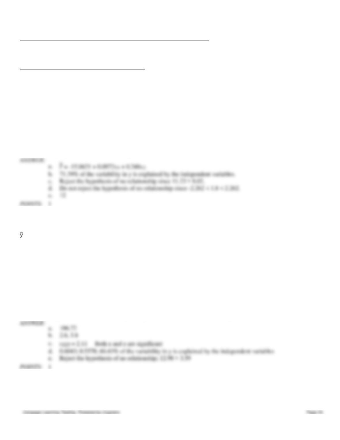
Write the estimated regression equation for the relationship between the variables.
b.
What can you say about the strength of this relationship?
c.
Carry out a test of whether y is significantly related to the independent variables. Use a .01
level of significance.
d.
Carry out a test of whether x1 and y are significantly related. Use a .05 level of significance.
e.
How many supermarkets are in the sample used here?
b.
71.39% of the variability in y is explained by the independent variables.
c.
Reject the hypothesis of no relationship since 11.23 > 8.02.
d.
e.
12
1
101. A regression was performed on a sample of 20 observations. Two independent variables were included in the
analysis, x and z. The relationship between x and z is z = x2. The following estimated equation was obtained.
= 23.72 + 12.61x + 0.798z
The standard errors for the coefficients are Sb1 = 4.85 and Sb2 = 0.21
For this model, SSR = 520.2 and SSE = 340.6
a.
Estimate the value of y when x = 5.
b.
Compute the appropriate t ratios.
c.
Test for the significance of the coefficients at the 5% level. Which variable(s) is (are)
significant?
d.
Compute the coefficient of determination and the adjusted coefficient of determination.
Interpret the meaning of the coefficient of determination.
e.
Test the significance of the relationship among the variables at the 5% level of significance.
a.
106.72
b.
2.6, 3.8
d.
0.6043; 0.5578; 60.43% of the variability in y is explained by the independent variables
e.
Reject the hypothesis of no relationship; 12.98 > 3.59
1
102. A student used multiple regression analysis to study how family spending (y) is influenced by income (x1), family
size (x2), and additions to savings (x3). The variables y, x1, and x3 are measured in thousands of dollars. The following
results were obtained.
Chapter 13 – Multiple Regression
ANOVA
df
SS
MS
F
Regression
3
45.9634
64.28
Error
11
2.6218
Coefficients
Standard Error
Intercept
0.0136
x1
0.7992
0.074
x2
0.2280
0.190
x3
-0.5796
0.920
Coefficient of determination = 0.946
a.
Write out the estimated regression equation for the relationship between the variables.
b.
What can you say about the strength of this relationship?
c.
Carry out a test of whether y is significantly related to the independent variables. Use a .05
level of significance.
d.
Carry out a test to see if x3 and y are significantly related. Use a .05 level of significance.
e.
Why would a coefficient of determination very close to 1.0 be expected here?
b.
94.6% of the variability in y is explained by the independent variables
c.
Reject the hypothesis of no relationship; 64.28 > 3.59
d.
Do not reject the hypothesis of no relationship; -2.201 < -0.63 < 2.201
y is x1 – x3
1
103. A regression model involving 3 independent variables for a sample of 20 periods resulted in the following sum of
squares.
Sum of
Squares
Regression
90
Residual (Error)
100
a.
Compute the coefficient of determination and fully explain its meaning.
b.
At α = 0.05 level of significance, test to determine whether or not there is a significant
relationship between the independent variables and the dependent variable.
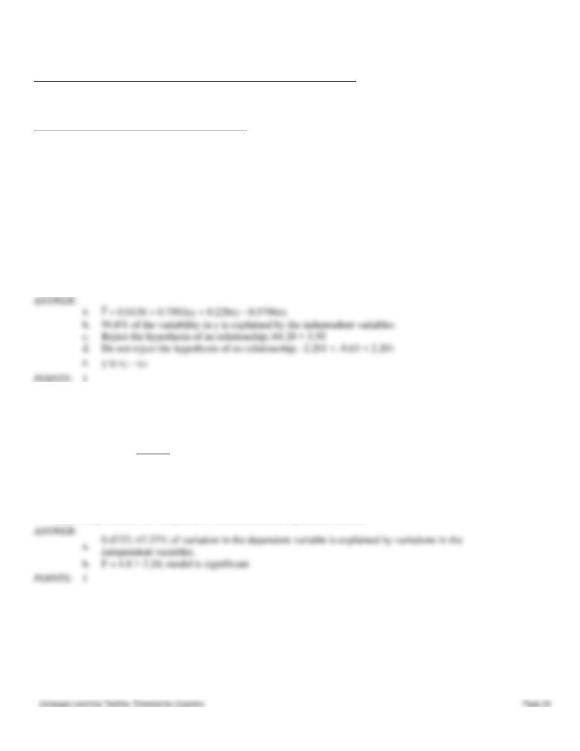
a.
0.4737; 47.37% of variation in the dependent variable is explained by variations in the
b.
F = 4.8 > 3.24; model is significant
1
104. A regression model involving 8 independent variables for a sample of 69 periods resulted in the following sum of
squares.
SSE = 306
SST = 1800
a.
Compute the coefficient of determination.
b.
At α = 0.05, test to determine whether or not the model is significant.
Chapter 13 – Multiple Regression
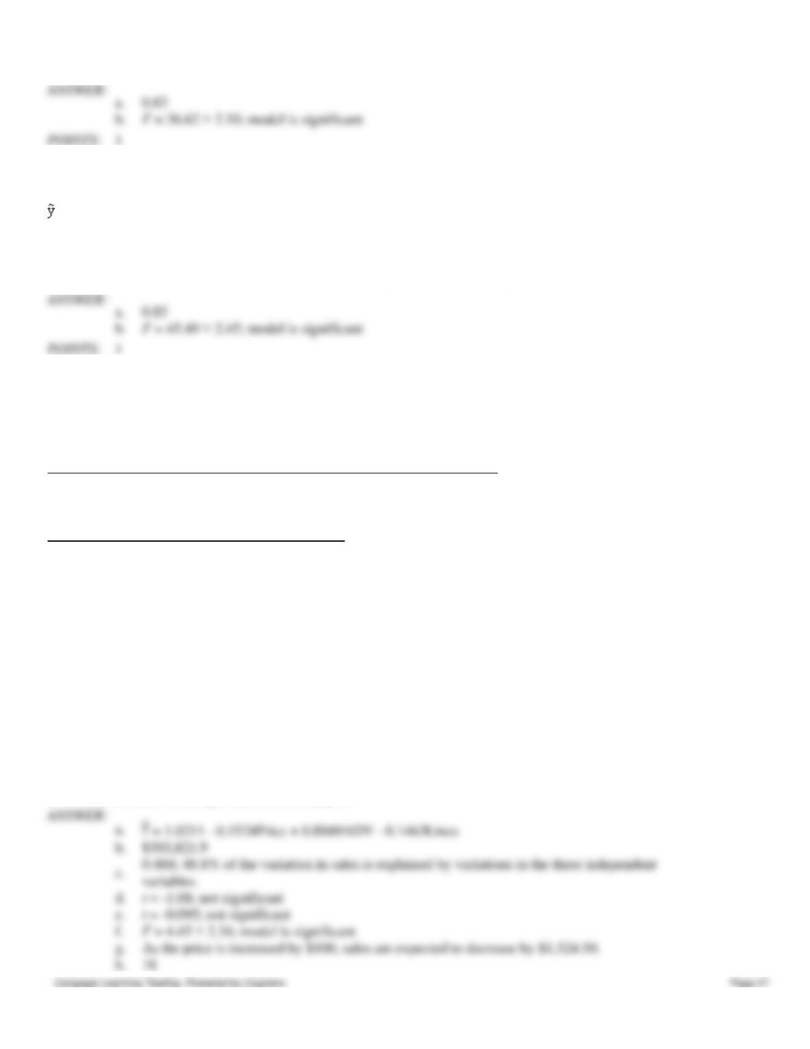
a.
0.83
b.
105. In a regression model involving 46 observations, the following estimated regression equation was obtained.
= 17 + 4x1 – 3x2 + 8x3 + 5x4 + 8x5
For this model, SST = 3410 and SSE = 510.
a.
Compute the coefficient of determination.
b.
Perform an F test and determine whether or not the regression model is significant.
a.
0.85
b.
106. A microcomputer manufacturer has developed a regression model relating his sales (y in $10,000s) with three
independent variables. The three independent variables are price per unit (Price in $100s), advertising (ADV in $1,000s)
and the number of product lines (Lines). Part of the regression results is shown below.
ANOVA
df
SS
MS
F
Regression
2708.61
Error
14
2840.51
Coefficients
Standard Error
Intercept
1.0211
22.8752
Price
-0.1524
0.1411
ADV
0.8849
0.2886
Lines
-0.1463
1.5340
a.
Use the above results and write the regression equation that can be used to predict sales.
b.
If the manufacturer has 10 product lines, advertising of $40,000, and the price per unit is
$3,000, what is your estimate of their sales? Give your answer in dollars.
c.
Compute the coefficient of determination and fully interpret its meaning.
d.
At α = 0.05, test to see if there is a significant relationship between sales and unit price.
e.
At α = 0.05, test to see if there is a significant relationship between sales and the number of
product lines.
f.
Is the regression model significant? (Perform an F test.)
g.
Fully interpret the meaning of the regression (coefficient of price) per unit that is, the slope for
the price per unit.
h.
What has been the sample size for this analysis?
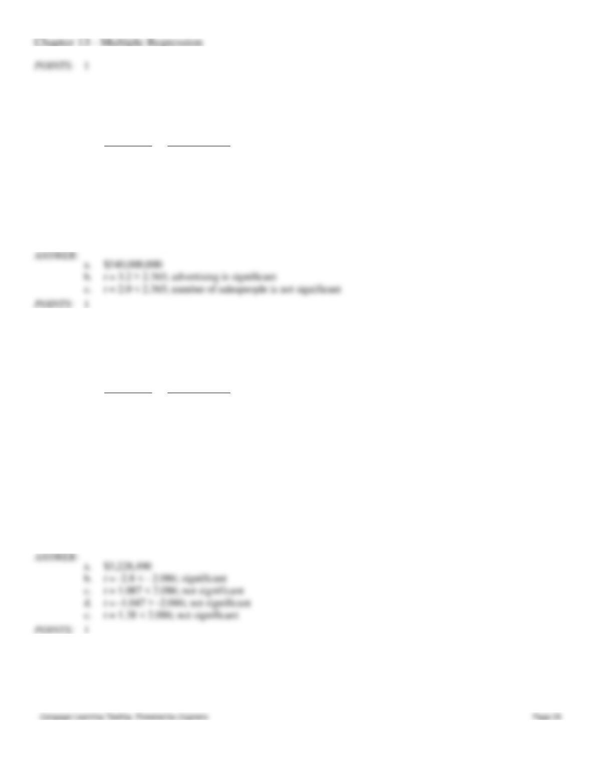
b.
$303,821.9
c.
0.488; 48.8% of the variation in sales is explained by variations in the three independent
d.
e.
f.
g.
As the price is increased by $100, sales are expected to decrease by $1,524.50.
h.
18
107. The following is part of the results of a regression analysis involving sales (y in millions of dollars), advertising
expenditures (x1 in thousands of dollars), and number of salespeople (x2) for a corporation. The regression was performed
on a sample of 10 observations.
Coefficient
Standard Error
Intercept
40.00
7.00
x1
8.00
2.50
x2
6.00
3.00
a.
If the company uses $40,000 in advertisement and has 30 salespersons, what are the expected
sales? Give your answer in dollars.
b.
At α = 0.05, test for the significance of the coefficient of advertising.
c.
At α = 0.05, test for the significance of the coefficient of the number of salespeople.
a.
$540,000,000
b.
c.
108. The Natural Drink Company has developed a regression model relating its sales (y in $10,000s) with four
independent variables. The four independent variables are price per unit (PRICE, in dollars), competitor’s price
(COMPRICE, in dollars), advertising (ADV, in $1,000s) and type of container used (CONTAIN; 1 = Cans and 0 =
Bottles). Part of the regression results is shown below. (Assume n = 25)
Coefficient
Standard Error
Intercept
443.143
PRICE
-57.170
20.426
COMPRICE
27.681
19.991
ADV
0.025
0.023
CONTAIN
-95.353
91.027
a.
If the manufacturer uses can containers, his price is $1.25, advertising $200,000, and his
competitor’s price is $1.50, what is your estimate of his sales? Give your answer in dollars.
b.
Test to see if there is a significant relationship between sales and unit price. Let α = 0.05.
c.
Test to see if there is a significant relationship between sales and advertising. Let α = 0.05.
d.
Is the type of container a significant variable? Let α = 0.05.
e.
Test to see if there is a significant relationship between sales and competitor’s price. Let α =
0.05.
a.
$3,228,490
b.
c.
d.
e.
109. The Very Fresh Juice Company has developed a regression model relating sales (y in $10,000s) with four
independent variables. The four independent variables are price per unit (x1, in dollars), competitor’s price (x2, in dollars),
advertising (x3, in $1,000s) and type of container used (x4) (1 = Cans and 0 = Bottles). Part of the regression results are
shown below:
Chapter 13 – Multiple Regression
Source of
Variation
Degrees of
Freedom
Sum of
Squares
Mean
Square
F
Regression
4
283,940.60
Error
18
621,735.14
Total
a.
Compute the coefficient of determination and fully interpret its meaning.
b.
Is the regression model significant? Explain what your answer implies. Let α = 0.05.
c.
What has been the sample size for this analysis?
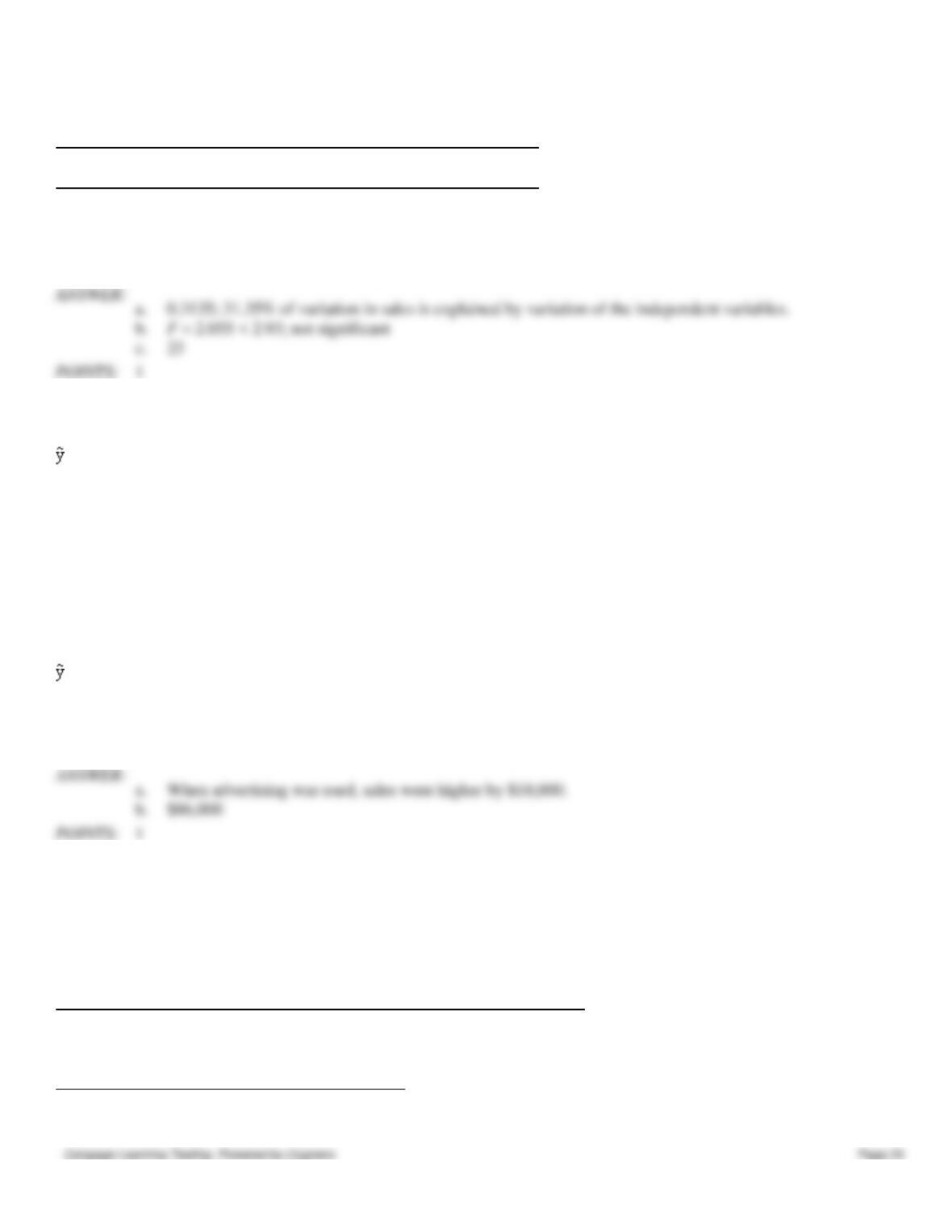
a.
0.3135; 31.35% of variation in sales is explained by variation of the independent variables.
b.
c.
23
1
110. The following regression model has been proposed to predict sales at a furniture store.
= 10 – 4x1 + 7x2 + 18x3
where
x1 = competitor’s previous day’s sales (in $1,000s)
x2 = population within 1 mile (in 1000s)
x3 = 1 if any form of advertising was used, 0 if otherwise
= sales (in $1,000s)
a.
Fully interpret the meaning of the coefficient of x3.
b.
Predict sales (in dollars) for a store with competitor’s previous day‘s sale of $3,000, a
population of 10,000 within 1 mile, and six radio advertisements.
a.
When advertising was used, sales were higher by $18,000.
b.
$86,000
1
111. A sample of 30 houses that were sold in the last year was taken. The value of the house (y) was estimated. The
independent variables included in the analysis were the number of rooms (x1), the size of the lot (x2), the number of
bathrooms (x3), and a dummy variable (x4), which equals 1 if the house has a garage and equals 0 if the house does not
have a garage. The following results were obtained:
ANOVA
df
SS
MS
F
Regression
204,242.88
51,060.72
Error
205,890.00
8,235.60
Coefficients
Standard Error
Intercept
15,232.5
8,462.5
x1
2,178.4
778.0
x2
7.8
2.2
x3
2,675.2
2,229.3
x4
1,157.8
463.1
a.
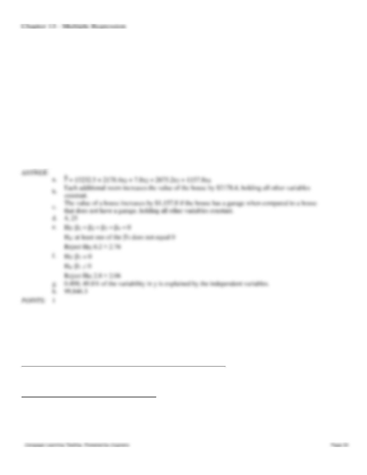
Write out the estimated equation.
b.
Interpret the coefficient on the number of rooms (x1).
c.
Interpret the coefficient on the dummy variable (x4).
d.
What are the degrees of freedom for the sum of squares explained by the regression (SSR) and
the sum of squares due to error (SSE)?
e.
Test whether or not there is a significant relationship between the value of a house and the
independent variables. Use a .05 level of significance. Be sure to state the null and alternative
hypotheses.
f.
Test the significance of β1 at the 5% level. Be sure to state the null and alternative hypotheses.
g.
Compute the coefficient of determination and interpret its meaning.
h.
Estimate the value of a house that has 9 rooms, a lot with an area of 7,500, 2 bathrooms, and a
garage.
a.
b.
Each additional room increases the value of the house by $2178.4, holding all other variables
The value of a house increases by $1,157.8 if the house has a garage when compared to a house
d.
4, 25
e.
Reject H0; 6.2 > 2.76
f.
Reject H0; 2.8 > 2.06
g.
0.498; 49.8% of the variability in y is explained by the independent variables.
h.
99,846.3
112. A sample of 25 families was taken. The objective of the study was to estimate the factors that determine the monthly
expenditure on food for families. The independent variables included in the analysis were the number of members in the
family (x1), the number of meals eaten outside the home (x2), and a dummy variable (x3) that equals 1 if a family member
is on a diet and equals 0 if there is no family member on a diet. The following results were obtained.
ANOVA
df
SS
MS
F
Regression
3,078.39
1,026.13
Error
2,013.90
95.90
Coefficients
Standard Error
Intercept
150.08
53.6
x1
49.92
9.6
x2
10.12
2.2
x3
-.60
12.0
Chapter 13 – Multiple Regression
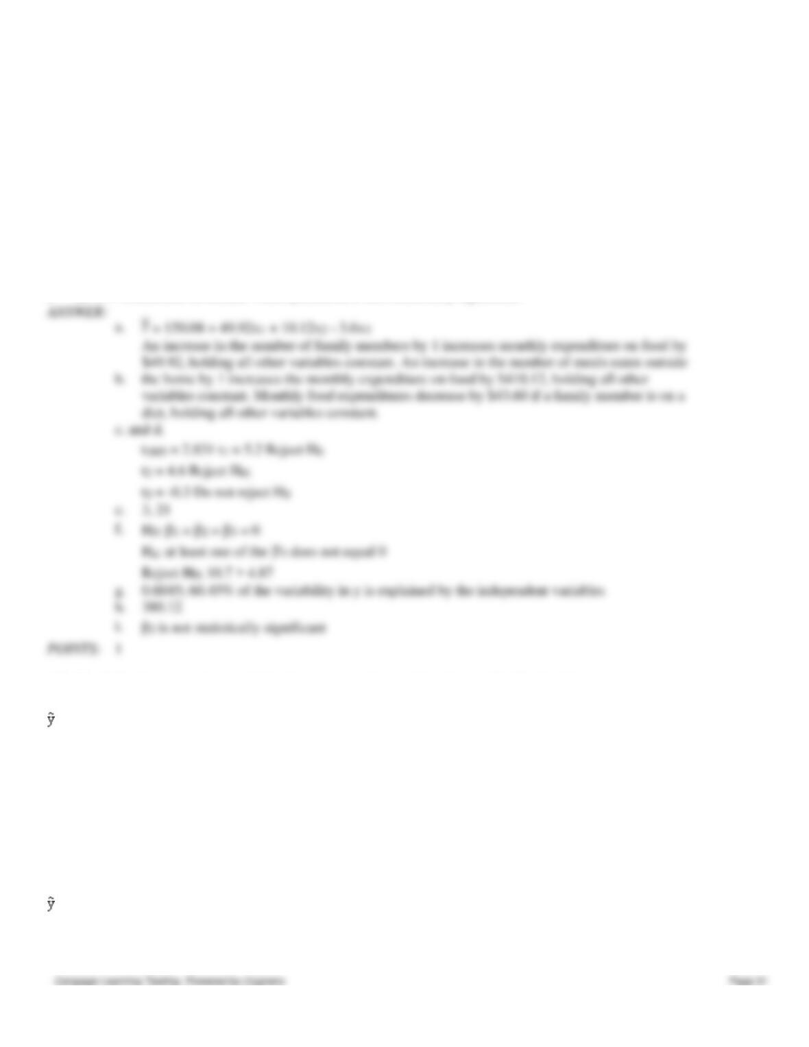
a.
Write out the estimated regression equation.
b.
Interpret all coefficients.
c.
Compute the appropriate t ratios.
d.
Test for the significance of β1, β2, and β3 at the 1% level of significance.
e.
What are the degrees of freedom for the sum of squares explained by the regression (SSR) and
the sum of squares due to error (SSE)?
f.
Test whether of not there is a significant relationship between the monthly expenditure on food
and the independent variables. Use a .01 level of significance. Be sure to state the null and
alternative hypotheses.
g.
Compute the coefficient of determination and explain its meaning.
h.
Estimate the monthly expenditure on food for a family that has 4 members, eats out 3 times,
and does not have any member of the family on a diet.
i.
At 95% confidence determine which parameter is not statistically significant.
the home by 1 increases the monthly expenditure on food by $410.12, holding all other
variables constant. Monthly food expenditures decrease by $43.60 if a family member is on a
c. and d.
e.
3, 21
g.
0.6045; 60.45% of the variability in y is explained by the independent variables
h.
113. The following regression model has been proposed to predict sales at a fast food outlet.
= 18 – 2x1 + 7x2 + 15x3
where
x1 = the number of competitors within 1 mile
x2 = the population within 1 mile (in 1,000s)
x3 = 1 if drive-up windows are present, 0 otherwise
= sales (in $1,000s)
a.
What is the interpretation of 15 (the coefficient of x3) in the regression equation?
b.
Predict sales for a store with 2 competitors, a population of 10,000 within one mile, and one
Chapter 13 – Multiple Regression
drive-up window (give the answer in dollars).
c.
Predict sales for the store with 2 competitors, a population of 10,000 within one mile, and no
drive-up window (give the answer in dollars).
Sales of stores with drive-up windows are $15,000 higher than those without drive-up
$99,000
$84,000
114. The following regression model has been proposed to predict sales at a computer store.
= 50 – 3x1 + 20x2 + 10x3
where
x1 = competitor’s previous day’s sales (in $1,000s)
x2 = population within 1 mile (in 1,000s)
= sales (in $1000s)
Predict sales (in dollars) for a store with the competitor’s previous day’s sale of $5,000, a population of 20,000 within 1
mile, and nine radio advertisements.
$445,000
115. The following regression model has been proposed to predict monthly sales at a shoe store.
= 40 – 3x1 + 12x2 + 10x3
where
x1 = competitor’s previous month’s sales (in $1,000s)
x2 = Stores previous month’s sales (in $1,000s)
= sales (in $1000s)
a.
Predict sales (in dollars) for the shoe store if the competitor’s previous month‘s sales were
$9,000, the store’s previous month’s sales were $30,000, and no radio advertisements were run.
b.
Predict sales (in dollars) for the shoe store if the competitor’s previous month‘s sales were
$9,000, the store’s previous month’s sales were $30,000, and 10 radio advertisements were run.
Chapter 13 – Multiple Regression
116. A company has recorded data on the weekly sales for its product (y), the unit price of the competitor’s product (x1),
and advertising expenditures (x2). The data resulting from a random sample of 7 weeks follows. Use Excel‘s Regression
Tool to answer the following questions.
Week
Price
Advertising
Sales
1
.33
5
20
2
.25
2
14
3
.44
7
22
4
.40
9
21
5
.35
4
16
6
.39
8
19
7
.29
9
15
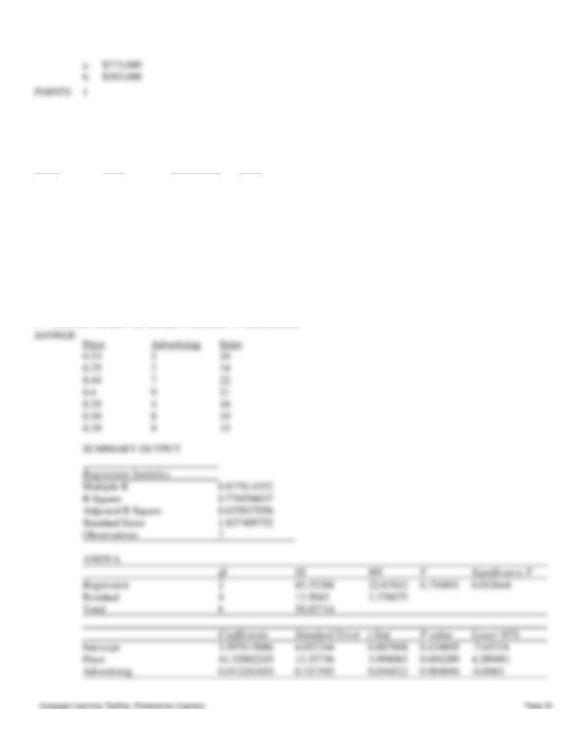
a.
What is the estimated regression equation?
b.
Determine whether the model is significant overall. Use α = 0.10.
c.
Determine if price is significantly related to sales. Use α = 0.10.
d.
Determine if advertising is significantly related to sales. Use α = 0.10.
e.
Find and interpret the multiple coefficient of determination.
Price
Advertising
Sales
0.33
5
20
0.25
2
14
0.44
7
22
0.35
4
16
0.39
8
19
0.29
9
15
SUMMARY OUTPUT
Multiple R
0.877814352
R Square
0.770558037
Adjusted R Square
0.655837056
Standard Error
1.837409752
Observations
7
ANOVA
Regression
2
45.35284
22.67642
6.716801
0.052644
Residual
4
13.5043
3.376075
Total
6
58.85714
Intercept
3.597615086
4.052244
0.887808
0.424805
-7.65324
Price
41.32002219
13.33736
3.098065
0.036289
4.289491
Advertising
0.013241819
0.327592
0.040422
0.969694
-0.8963
a.
$373,000
b.
$383,000
1
Chapter 13 – Multiple Regression
117. The prices of Rawlston, Inc. stock (y) over a period of 12 days, the number of shares (in 100s) of company’s stocks
sold (x1), and the volume of exchange (in millions) on the New York Stock Exchange (x2) are shown below.
Day
y
x1
x2
1
87.50
950
11.00
2
86.00
945
11.25
3
84.00
940
11.75
4
83.00
930
11.75
5
84.50
935
12.00
6
84.00
935
13.00
7
82.00
932
13.25
8
80.00
938
14.50
9
78.50
925
15.00
10
79.00
900
16.50
11
77.00
875
17.00
12
77.50
870
17.50
Excel was used to determine the least-squares regression equation. Part of the computer output is shown below.
ANOVA
df
SS
MS
F
Significance F
Regression
2
118.8474
59.4237
40.9216
0.0000
Residual
9
13.0692
1.4521
Total
11
131.9167
Coefficients
Standard Error
t Stat
P-value
Intercept
118.5059
33.5753
3.5296
0.0064
x1
-0.0163
0.0315
-0.5171
0.6176
x2
-1.5726
0.3590
-4.3807
0.0018
a.
Use the output shown above and write an equation that can be used to predict the price of the
stock.
b.
Interpret the coefficients of the estimated regression equation that you found in Part a.
c.
At 95% confidence, determine which variables are significant and which are not.
d.
If in a given day, the number of shares of the company that were sold was 94,500 and the
volume of exchange on the New York Stock Exchange was 16 million, what would you
expect the price of the stock to be?
e.
POINTS:
1