True or False: TABLE 17-9
What are the factors that determine the acceleration time (in sec.) from 0 to 60 miles per
hour of a car? Data on the following variables for 171 different vehicle models were
collected:
Accel Time: Acceleration time in sec.
Cargo Vol: Cargo volume in cu. ft.
HP: Horsepower
MPG: Miles per gallon
SUV: 1 if the vehicle model is an SUV with Coupe as the base when SUV and Sedan
are both 0
Sedan: 1 if the vehicle model is a sedan with Coupe as the base when SUV and Sedan
are both 0
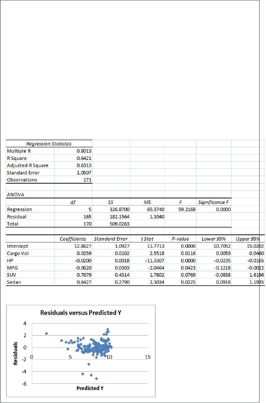
The regression results using acceleration time as the dependent variable and the
remaining variables as the independent variables are presented below.
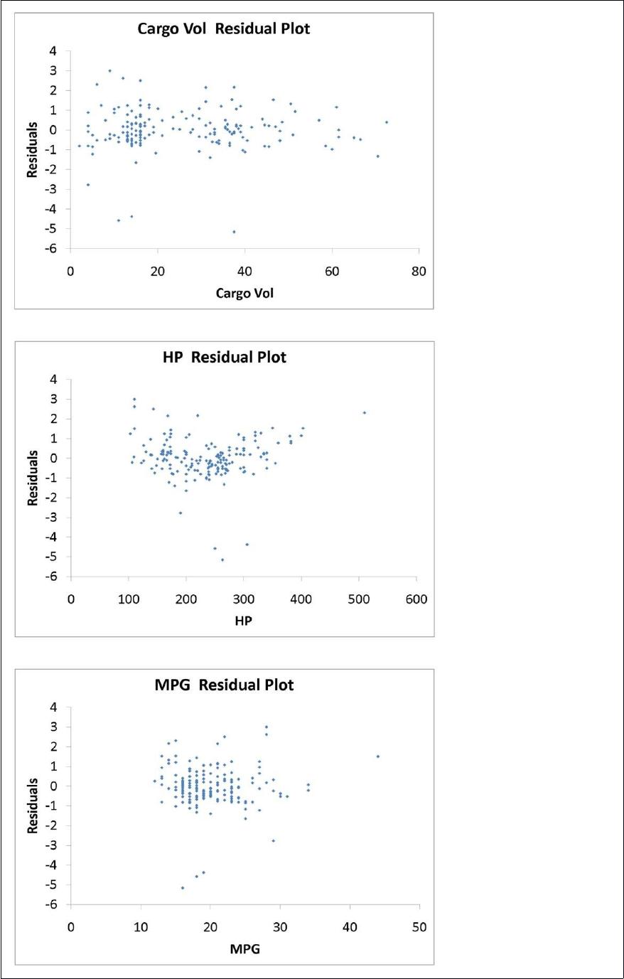
The various residual plots are as shown below.
The coefficient of partial determination ( ) of each of the 5
predictors are, respectively, 0.0380, 0.4376, 0.0248, 0.0188, and 0.0312.
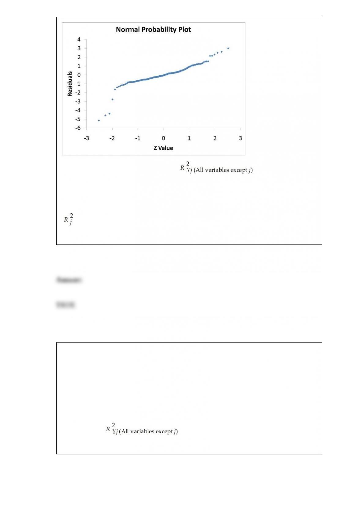
The coefficient of multiple determination for the regression model using each of the 5
variables Xj as the dependent variable and all other X variables as independent variables
( ) are, respectively, 0.7461, 0.5676, 0.6764, 0.8582, 0.6632.
Referring to Table 17-9, the error appears to be left-skewed.
True or False: TABLE 17-10
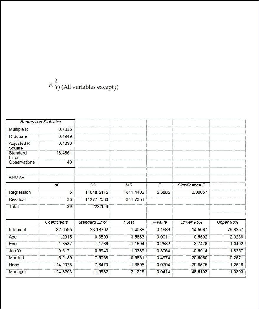
Given below are results from the regression analysis where the dependent variable is
the number of weeks a worker is unemployed due to a layoff (Unemploy) and the
independent variables are the age of the worker (Age), the number of years of education
received (Edu), the number of years at the previous job (Job Yr), a dummy variable for
marital status (Married: 1 = married, 0 = otherwise), a dummy variable for head of
household (Head: 1 = yes, 0 = no) and a dummy variable for management position
(Manager: 1 = yes, 0 = no). We shall call this Model 1. The coefficient of partial
determination ( ) of each of the 6 predictors are, respectively,
0.2807, 0.0386, 0.0317, 0.0141, 0.0958, and 0.1201.
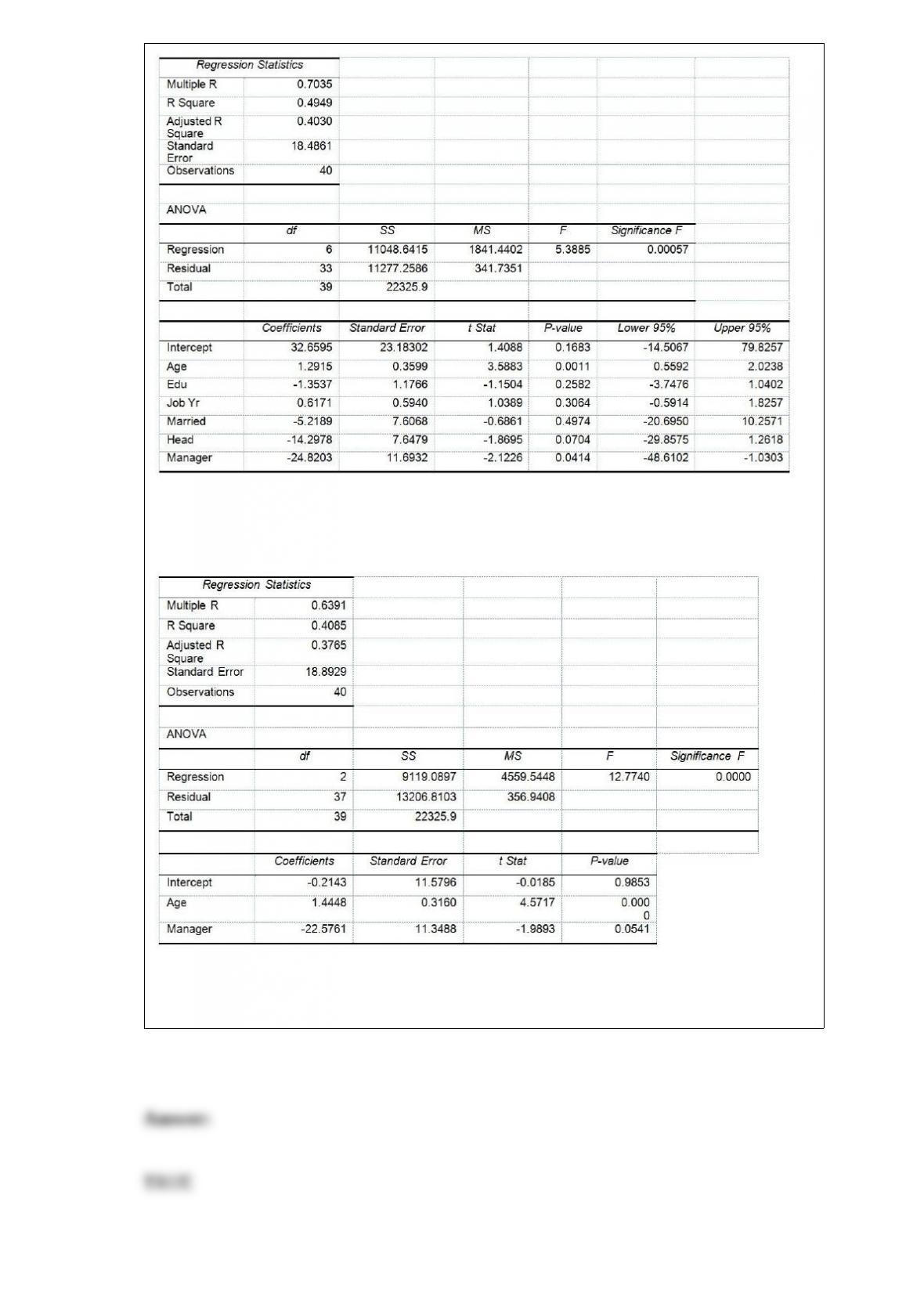
Model 2 is the regression analysis where the dependent variable is Unemploy and the
independent variables are Age and Manager. The results of the regression analysis are
given below:
Referring to Table 17-10, Model 1, the null hypothesis should be rejected at a 10% level
of significance when testing whether age has any effect on the number of weeks a
worker is unemployed due to a layoff.

TABLE 14-17
Given below are results from the regression analysis where the
dependent variable is the number of weeks a worker is unemployed
due to a layo! (Unemploy) and the independent variables are the age
of the worker (Age) and a dummy variable for management position
(Manager: 1 = yes, 0 = no).
The results of the regression analysis are given below:
True or False: Referring to Table 14-17, we can conclude that, holding
constant the e!ect of the other independent variable, there is a
di!erence in the mean number of weeks a worker is unemployed due
to a layo! between a worker who is in a management position and
one who is not at a 5% level of signiticance if we use only the
information of the 95% confidence interval estimate for the di!erence
in the mean number of weeks a worker is unemployed due to a layo!
between a worker who is in a management position and one who is
not.

TABLE 14-15
The superintendent of a school district wanted to predict the
percentage of students passing a sixth-grade proficiency test. She
obtained the data on percentage of students passing the proficiency
test (% Passing), mean teacher salary in thousands of dollars
(Salaries), and instructional spending per pupil in thousands of dollars
(Spending) of 47 schools in the state.
Following is the multiple regression output with Y = % Passing as the
dependent variable, X1 = Salaries and X2 = Spending:
True or False: Referring to Table 14-15, you can conclude that mean
teacher salary has no impact on the mean percentage of students
passing the proficiency test, taking into account the e!ect of
instructional spending per pupil, at a 5% level of signiticance using
the confidence interval estimate for β1.
True or False: TABLE 17-10
Given below are results from the regression analysis where the dependent variable is
the number of weeks a worker is unemployed due to a layoff (Unemploy) and the
independent variables are the age of the worker (Age), the number of years of education
received (Edu), the number of years at the previous job (Job Yr), a dummy variable for
marital status (Married: 1 = married, 0 = otherwise), a dummy variable for head of
household (Head: 1 = yes, 0 = no) and a dummy variable for management position
(Manager: 1 = yes, 0 = no). We shall call this Model 1. The coefficient of partial
determination ( ) of each of the 6 predictors are, respectively,
0.2807, 0.0386, 0.0317, 0.0141, 0.0958, and 0.1201.
Model 2 is the regression analysis where the dependent variable is Unemploy and the
independent variables are Age and Manager. The results of the regression analysis are
given below:

Referring to Table 17-10 and using both Model 1 and Model 2, the null hypothesis for
testing whether the independent variables that are not significant individually are also
not significant as a group in explaining the variation in the dependent variable should
be rejected at a 5% level of significance.
TABLE 14-18
A logistic regression model was estimated in order to predict the
probability that a randomly chosen university or college would be a
private university using information on mean total Scholastic Aptitude
Test score (SAT) at the university or college and whether the TOEFL
criterion is at least 90 (Toe90 = 1 if yes, 0 otherwise). The
dependent variable, Y, is school type (Type = 1 if private and 0
otherwise).
The PHStat output is given below:

True or False: Referring to Table 14-18, there is not enough evidence
to conclude that Toe90 makes a signiticant contribution to the
model in the presence of SAT at a 0.05 level of signiticance.
True or False: A sample is used to obtain a 95% confidence interval for the mean of a
population. The confidence interval goes from 15 to 19. If the same sample had been
used to test the null hypothesis that the mean of the population is equal to 20 versus the
alternative hypothesis that the mean of the population differs from 20, the null
hypothesis could be rejected at a level of significance of 0.02.
TABLE 8-8
The president of a university would like to estimate the proportion of the student
population that owns a personal computer. In a sample of 500 students, 417 own a
personal computer.
True or False: Referring to Table 8-8, we are 99% confident that the mean numbers of
student population who own a personal computer is between 0.7911 and 0.8769.

True or False: The Laspeyres price index uses the initial consumption quantities as the
weights.
True or False: If you are comparing the mean sales among 3 different brands, you are
dealing with a three-way ANOVA design.
True or False: Opportunity loss is the difference between the lowest profit for an event
and the actual profit obtained for an action taken.
TABLE 7-8
According to a survey, only 15% of customers who visited the website of a major retail

store made a purchase. Random samples of size 50 are selected from a population of
900. Use the finite population correction factor.
True or False: Referring to Table 7-8, the requirements for using a normal distribution
to approximate a binomial distribution is fulfilled.
True or False: Given a sample mean of 2.1 and a sample standard deviation of 0.7 from
a sample of 10 data points, a 90% confidence interval will have a width of 2.36.
True or False: The Cpk is a one-sided specification limit.
TABLE 2-11
The ordered array below resulted from selecting a sample of 25 batches of 500
computer chips and determining how many in each batch were defective.
Defects

Referring to Table 2-11, construct a histogram for the defects data, using “0 but less
than 5″ as the first class.
TABLE 9-10
A manufacturer produces light bulbs that have a mean life of at least 500 hours when
the production process is working properly. Based on past experience, the population
standard deviation is 50 hours and the light bulb life is normally distributed. The
operations manager stops the production process if there is evidence that the population
mean light bulb life is below 500 hours.
Referring to Table 9-10, if you select a sample of 100 light bulbs and are willing to have
a level of significance of 0.01, the probability of the operations manager not stopping
the process if the population mean bulb life is 510 hours is ________.
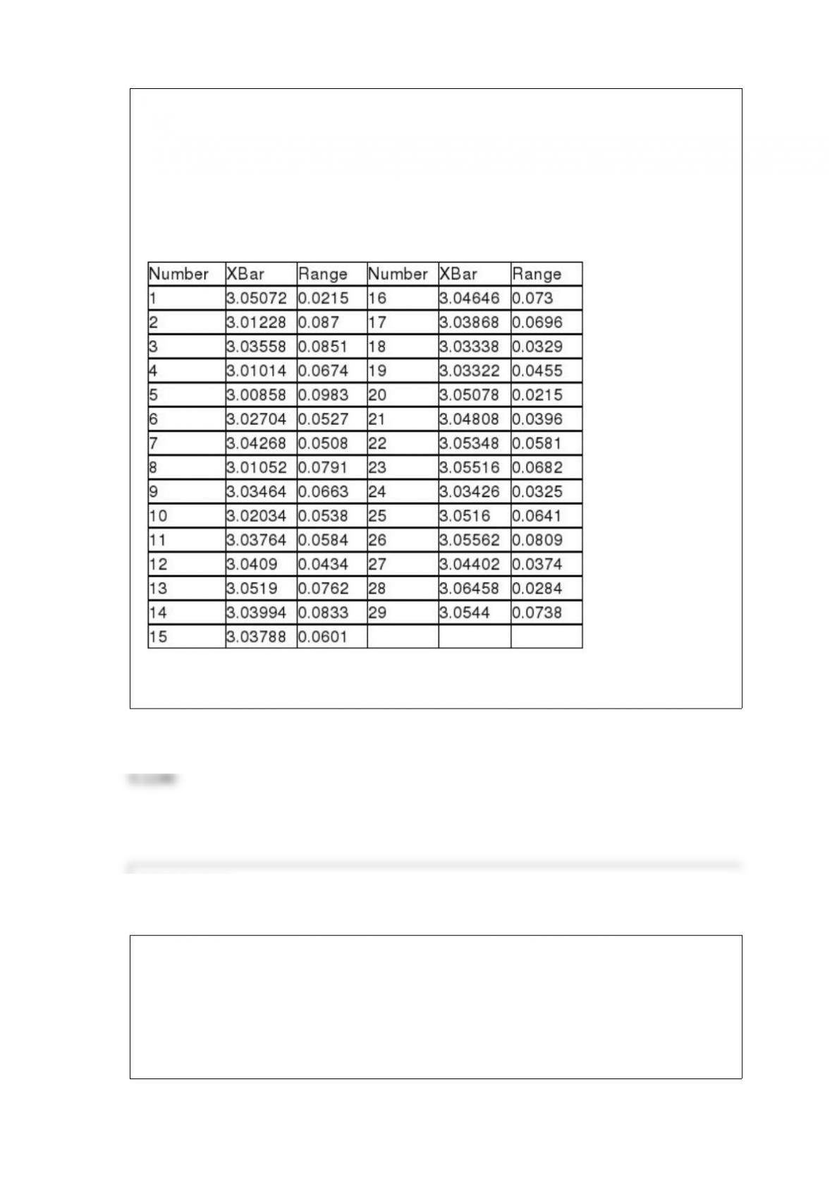
TABLE 18-9
The manufacturer of canned food constructed control charts and analyzed several
quality characteristics. One characteristic of interest is the weight of the filled cans. The
lower specification limit for weight is 2.95 pounds. The table below provides the range
and mean of the weights of five cans tested every fifteen minutes during a day’s
production.
Referring to Table 18-9, an R chart is to be constructed for the weight. The upper
control limit for this data set is ________.
TABLE 12-5
Four surgical procedures currently are used to install pacemakers. If the patient does not
need to return for follow-up surgery, the operation is called a “clear” operation. A heart
center wants to compare the proportion of clear operations for the 4 procedures, and
collects the following numbers of patients from their own records:
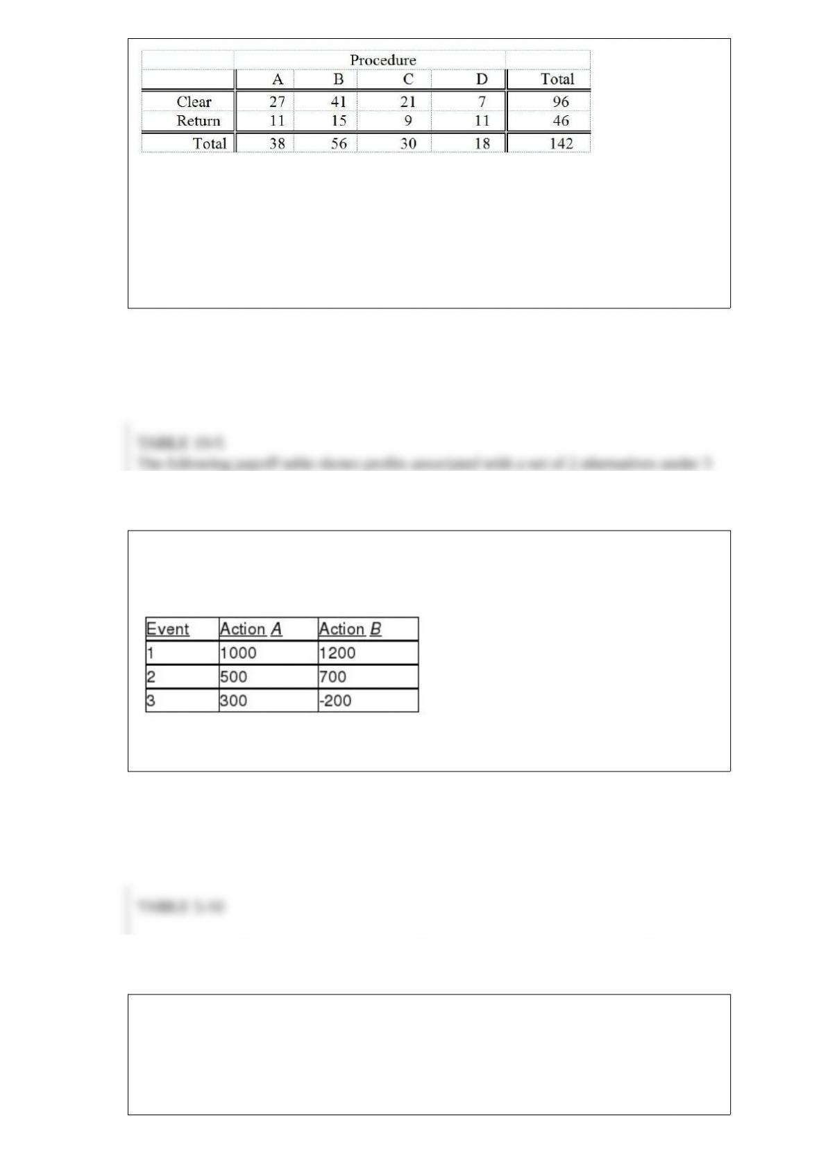
They will use this information to test for a difference among the proportion of clear
operations using a chi-square test with a level of significance of 0.05.
Referring to Table 12-5, what is the value of the critical range for the Marascuilo
procedure to test for the difference in proportions between procedure B and procedure
C using a 0.05 level of significance?
TABLE 19-5
The following payoff table shows profits associated with a set of 2 alternatives under 3
possible events.
Suppose that the probability of Event 1 is 0.2, Event 2 is 0.5, and Event 3 is 0.3.
Referring to Table 19-5, what is the optimal action using the return to risk ratio?
TABLE 5-10
An accounting firm in a college town usually recruits employees from two of the
universities in town. This year, there are fifteen graduates from University A and five
from University B and the firm decides to hire six new employees from the two

universities.
Referring to Table 5-10, what is the probability that all of the new employees will be
from University B?