20
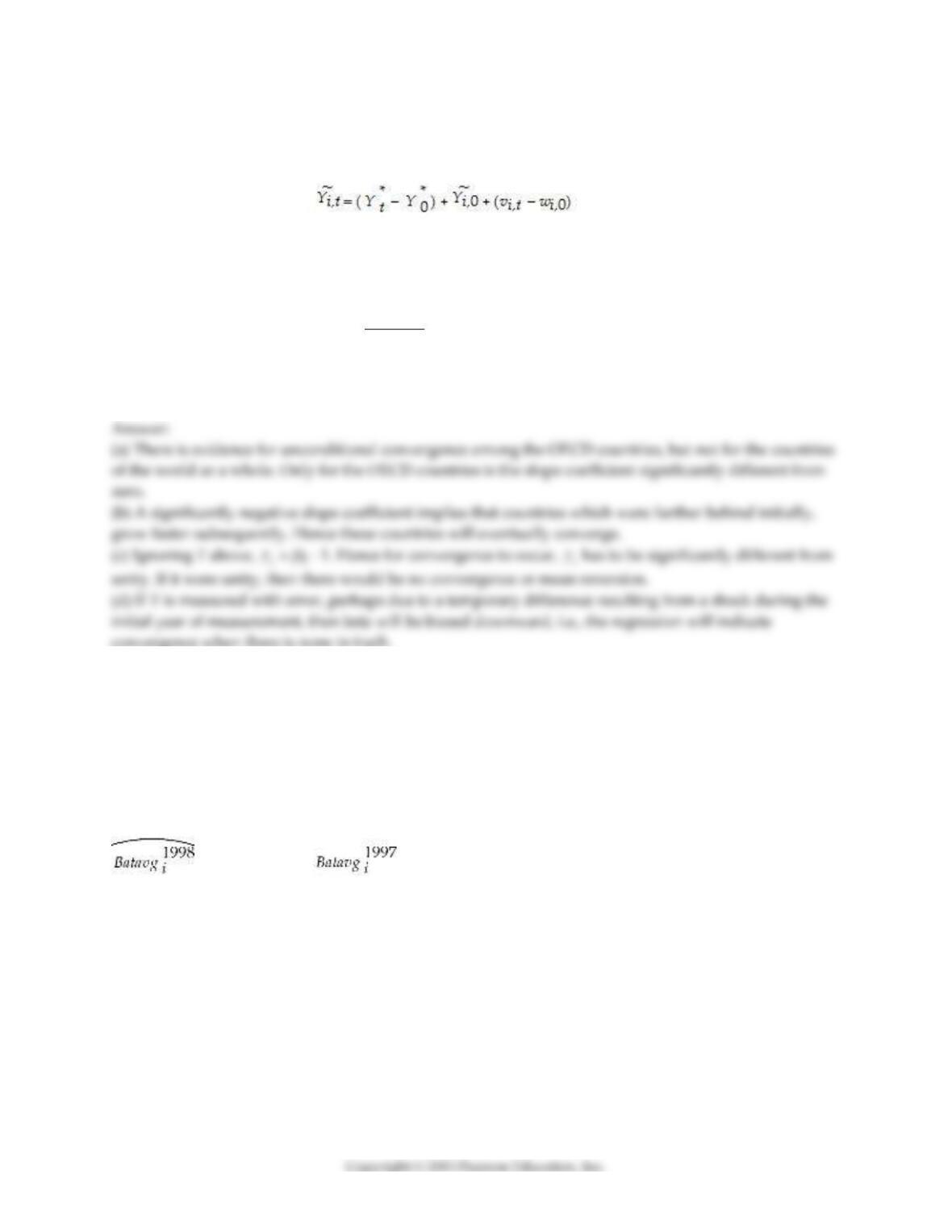
where the “*” variables represent true, or permanent, per capita income components, while v and w are
temporary or transitory components. Subtraction of the initial period from the current period then results
in
Ignoring, without loss of generality, the constant in the above equation, and making standard
assumptions about the error term, one can show that by regressing current per capita income on a
constant and the initial period per capita income, the slope behaves as follows:
2
122
ˆ1
pv
v
Y
⎯⎯→ − +
Discuss the implications for the convergence results above.
10) One of the most frequently used summary statistics for the performance of a baseball hitter is the so–
called batting average. In essence, it calculates the percentage of hits in the number of opportunities to hit
(appearances “at the plate”). The management of a professional team has hired you to predict next
season’s performance of a certain hitter who is up for a contract renegotiation after a particularly great
year. To analyze the situation, you search the literature and find a study which analyzed players who had
at least 50 at bats in 1998 and 1997. There were 379 such players.
(a) The reported regression line in the study is
= 0.138 + 0.467 × ; R2= 0.17
21
and the intercept and slope are both statistically significant. What does the regression imply about the
relationship between past performance and present performance? What values would the slope and
intercept have to take on for the future performance to be as good as the past performance, on average?
(b) Being somewhat puzzled about the results, you call your econometrics professor and describe the
results to her. She says that she is not surprised at all, since this is an example of “Galton’s Fallacy.” She
explains that Sir Francis Galton regressed the height of offspring on the mid–height of their parents and
found a positive intercept and a slope between zero and one. He referred to this result as “regression
towards mediocrity.” Why do you think econometricians refer to this result as a fallacy?
(c) Your professor continues by mentioning that this is an example of errors–in–variables bias. What does
she mean by that in general? In this case, why would batting averages be measured with error? Are
baseball statisticians sloppy?
(d) The top three performers in terms of highest batting averages in 1997 were Tony Gwynn (.372), Larry
Walker (.366), and Mike Piazza (.362). Given your answers for the previous questions, what would be
your predictions for the 1998 season?
11) Your textbook compares the results of a regression of test scores on the student–teacher ratio using a
sample of school districts from California and from Massachusetts. Before standardizing the test scores
for California, you get the following regression result:
= 698.9 – 2.28×STR
n = 420, R2 = 0.051, SER = 18.6
In addition, you are given the following information: the sample mean of the student–teacher ratio is
19.64 with a standard deviation of 1.89, and the standard deviation of the test scores is 19.05.
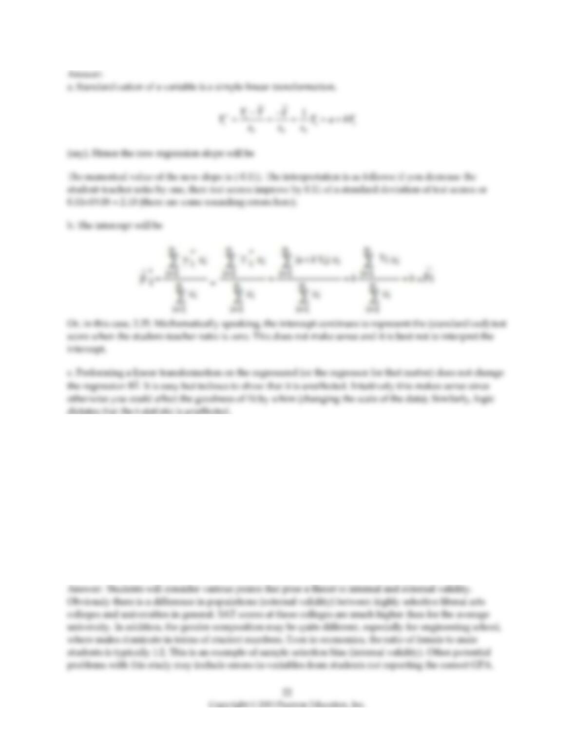
a. After standardizing the test scores variable and running the regression again, what is the value of the
slope? What is the meaning of this new slope here (interpret the result)?
b. What will be the new intercept? Now that test scores have been standardized, should you interpret the
intercept?
c. Does the regression R2 change between the two regressions? What about the t–statistic for the slope
estimator?
12) Suppose that you have just read a review of the literature of the effect of beauty on earnings. You
were initially surprised to find a mild effect of beauty even on teaching evaluations at colleges. Intrigued
by this effect, you consider explanations as to why more attractive individuals receive higher salaries.
One of the possibilities you consider is that beauty may be a marker of performance/productivity. As a
result, you set out to test whether or not more attractive individuals receive higher grades (cumulative
GPA) at college. You happen to have access to individuals at two highly selective liberal arts colleges
nearby. One of these specializes in Economics and Government and incoming students have an average
SAT of 2,100; the other is known for its engineering program and has an incoming SAT average of 2,200.
Conducting a survey, where you offer students a small incentive to answer a few questions regarding
their academic performance, and taking a picture of these individuals, you establish that there is no
relationship between grades and beauty. Write a short essay using some of the concepts of internal and
external validity to determine if these results are likely to apply to universities in general.
9.3 Mathematical and Graphical Problems
1) Your textbook gives the following example of simultaneous causality bias of a two equation system:
Yi = β0 + β1Xi + ui
Xi =
0
+
1
Yi + vi
In microeconomics, you studied the demand and supply of goods in a single market. Let the demand
() and supply ( ) for the i–th good be determined as follows,
= β0 – β1Pi + ui,
=
0
–
1
Pi + vi,
where P is the price of the good. In addition, you typically assume that the market clears.
Explain how the simultaneous causality bias applies in this situation. The textbook explained a positive
correlation between Xi and ui for
1
> 0 through an argument that started from “imagine that ui is
negative.” Repeat this exercise here.
2) The errors–in–variables model analyzed in the text results in
2
11
22
ˆpX
Xw
⎯⎯→ +
so that the OLS estimator is inconsistent. Give a condition involving the variances of X and w, under
which the bias towards zero becomes small.
3) You have been hired as a consultant by building contractor, who have been sued by the owners’
representatives of a large condominium project for shoddy construction work. In order to assess the
damages for the various units, the owners’ association sent out a letter to owners and asked if people
were willing to make their units available for destructive testing. Destructive testing was conducted in
some of these units as a result of the responses. Based on the tests, the owners‘ association inferred the
damage over the entire condo complex. Do you think that the inference is valid in this case? Discuss how
proper sampling should proceed in this situation.
4) Assume that a simple economy could be described by the following system of equations,
Ct = β0 + β1Yt + ui
It = ,
where C is consumption, Y is income, and I is investment. (This may be a primitive island society which
does not trade with other islands. There is no government, and the only good consumed and invested
(saved) is sunflower seeds.)
Assume the presence of the GDP identity, Y = C + I. If you estimated the consumption function, what sort
of problem involving internal validity may be present?
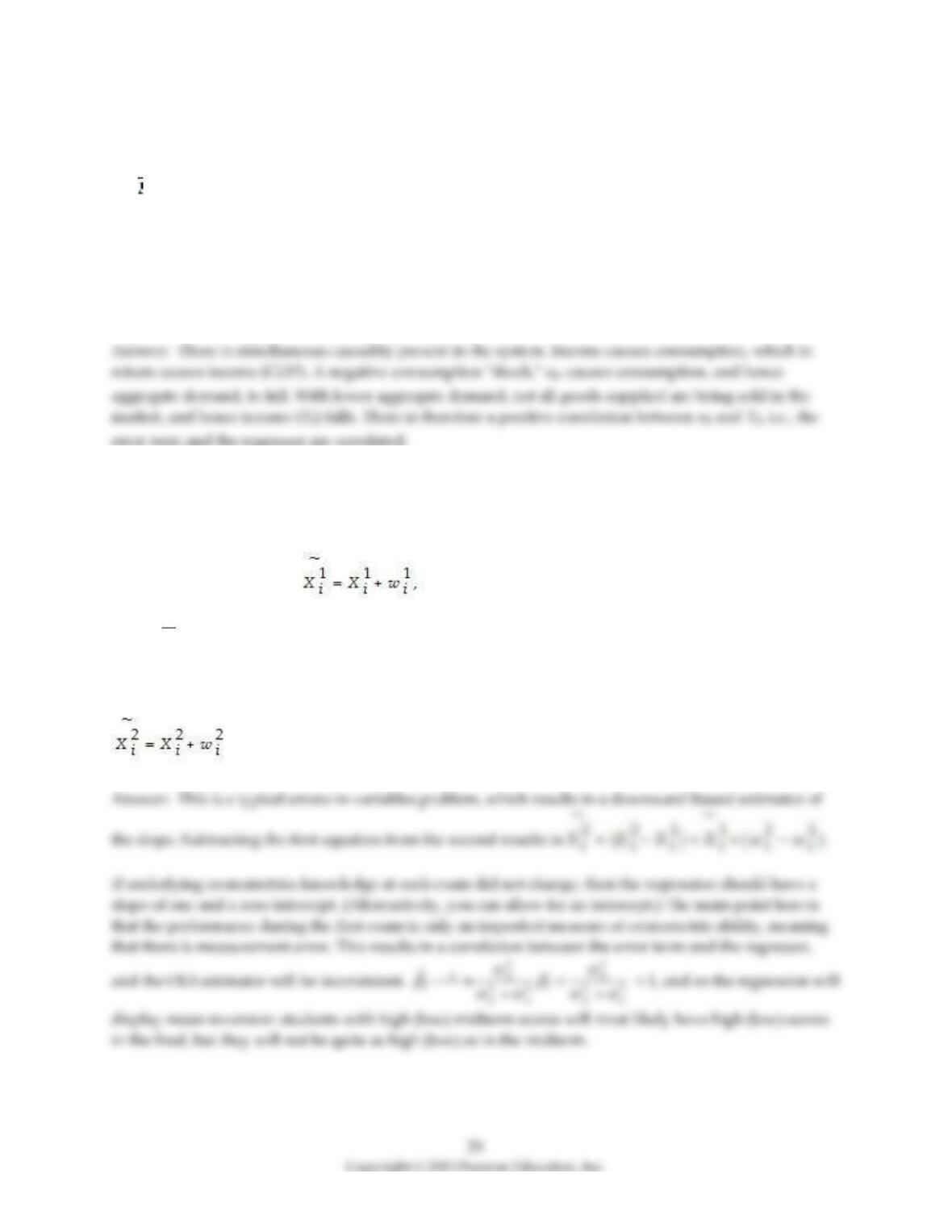
5) Your professor wants to measure the class’s knowledge of econometrics twice during the semester,
once in a midterm and once in a final. Assume that your performance, and that of your peers, on the day
of your midterm exam only measure knowledge imperfectly and with an error,
where
X
is your exam grade, X is underlying econometrics knowledge, and w is a random error with
mean zero and variance
2
w
. w may depend on whether you have a headache that day, whether or not the
questions you had prepared for appeared on the exam, your mood, etc. A similar situation holds for the
final, which is exam two:
. What would happen if you ran a regression of grades received by students in the final
on midterm grades?
26
6) Consider the one–variable regression model, Yi = β0 + β1Xi + ui, where the usual assumptions from
Chapter 4 are satisfied. However, suppose that both Y and X are measured with error, = Yi + zi and
= Xi + wi. Let both measurement errors be i.i.d. and independent of both Y and X respectively. If you
estimated the regression model = β0 + β1+ vi using OLS, then show that the slope estimator is not
consistent.
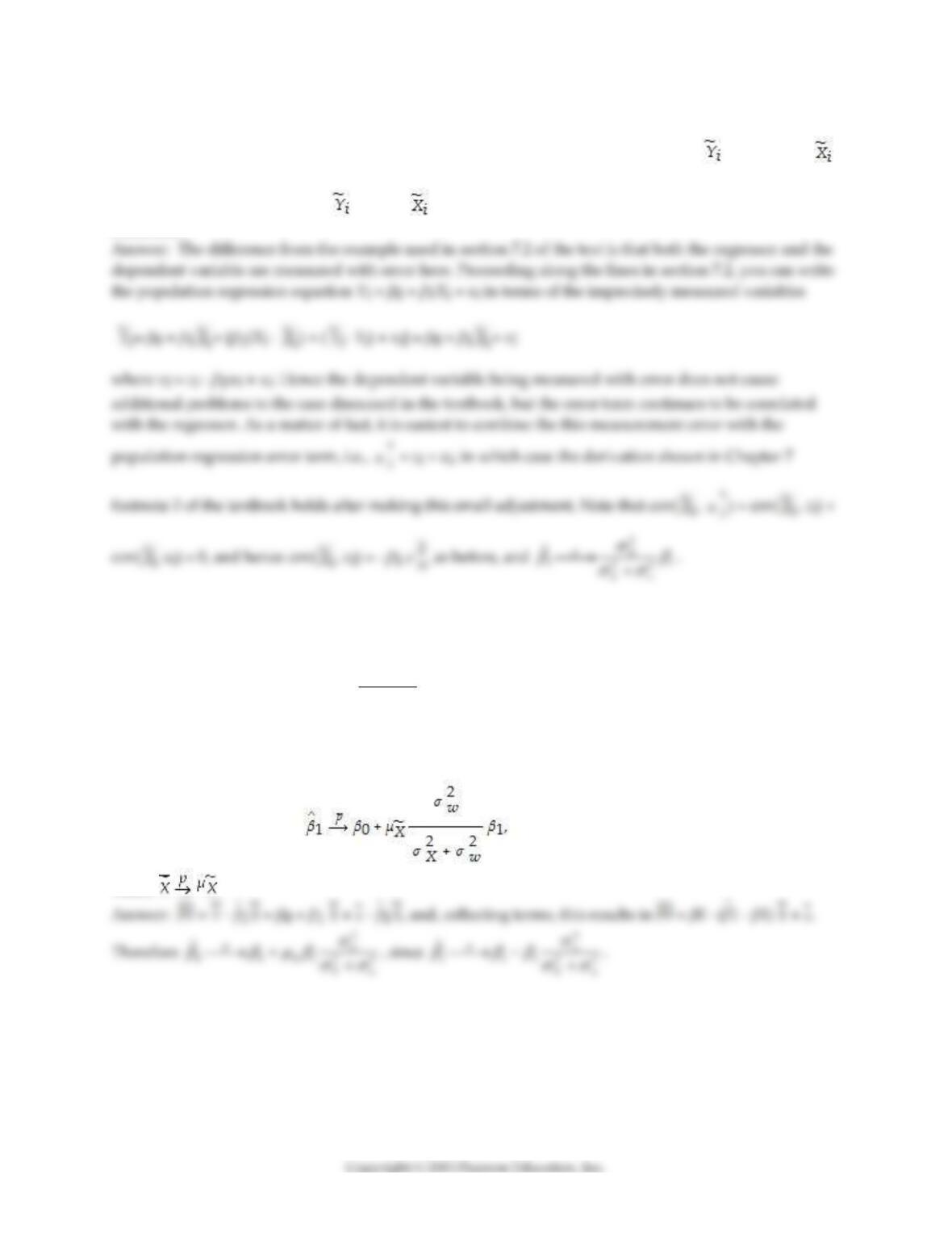
7) In the simple, one–explanatory variable, errors–in–variables model, the OLS estimator for the slope is
inconsistent. The textbook derived the following result
2
11
22
ˆpX
Xw
⎯⎯→ +
.
Show that the OLS estimator for the intercept behaves as follows in large samples:
where .
8) Assume that you had found correlation of the residuals across observations. This may happen because
the regressor is ordered by size. Your regression model could therefore be specified as follows:
Yi = β0 + β1Xi + ui
ui = ρui–1 + vi; < 1.
Furthermore, assume that you had obtained consistent estimates for β0, β1, ρ. If asked to make a
prediction for Y, given a value of X(= Xj) and j–1, how would you proceed? Would you use the
information on the lagged residual at all? Why or why not?
9) Your textbook only analyzed the case of an error–in–variables bias of the type i= Xi + wi. What if the
error were generated in the simple regression model by entering data that always contained the same
typographical error, say i= Xi + a or i= bXi, where a and b are constants. What effect would this have on
your regression model?
10) Explain why the OLS estimator for the slope in the simple regression model is still unbiased, even if
there is correlation of the error term across observations.
28
11) To analyze the situation of simultaneous causality bias, consider the following system of equations:
Yi = β0 + β1Xi + ui
Xi = + Yi + vi
Demonstrate the negative correlation between Xi and for < 0 , either through mathematics or by
presenting an argument which starts as follows: “Imagine that ui is negative.”
12) Think of three different economic examples where cross–sectional data could be collected. Indicate in
each of these cases how you would check if the analysis is externally valid.
13) The textbook derived the following result:
2
11
22
ˆpX
Xw
⎯⎯→ +
. Show that this is the same as
2
1 1 1
22
ˆpw
wX
⎯⎯→ +
.
14) Your textbook has analyzed simultaneous equation systems in the case of two equations,
Yi = β0 + β1Xi + ui
Xi = + Yi + vi,
where the first equation might be the labor demand equation (with capital stock and technology being
held constant), and the second the labor supply equation (X being the real wage, and the labor market
clears). What if you had a a production function as the third equation
Zi = + Yi + wi
where Z is output. If the error terms, u, v, and w, were pairwise uncorrelated, explain why there would be
no simultaneous causality bias when estimating the production function using OLS.
15) A professor in your microeconomics lectures derived a labor demand curve in the lecture. Given some
reasonable assumptions, she showed that the demand for labor depends negatively on the real wage. You
want to put this hypothesis to the test (“show me”) and collect data on employment and real wages for a
certain industry. You try to estimate the labor demand curve but find no relationship between the two
variables. Is economic theory wrong? Explain.
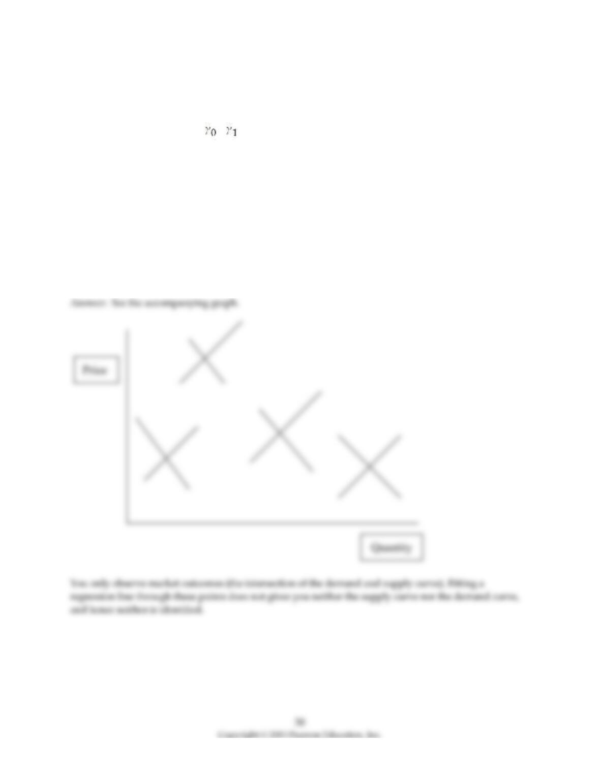
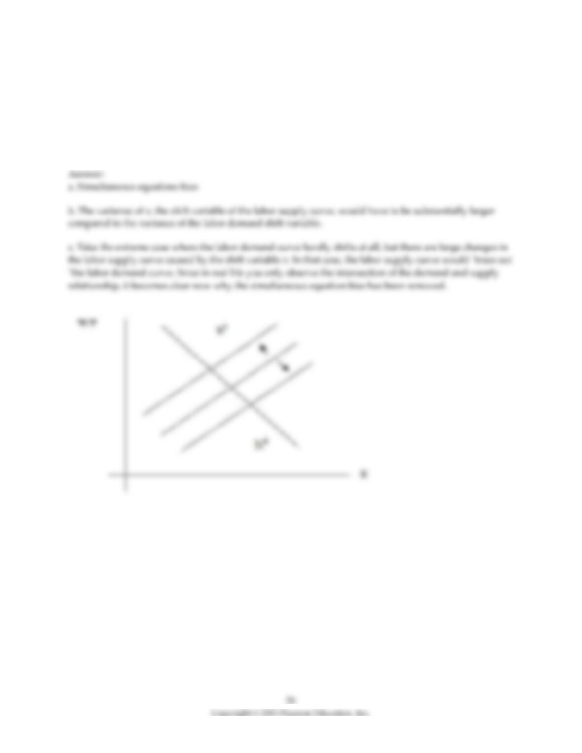
16) Your textbook uses the following example of simultaneous causality bias of a two equation system:
Yi = β0 + β1Xi + ui
Xi = + Yi + vi
To be more specific, think of the first equation as a demand equation for a certain good, where Y is the
quantity demanded and X is the price. The second equation then represents the supply equation, with a
third equation establishing that demand equals supply. Sketch the market outcome over a few periods
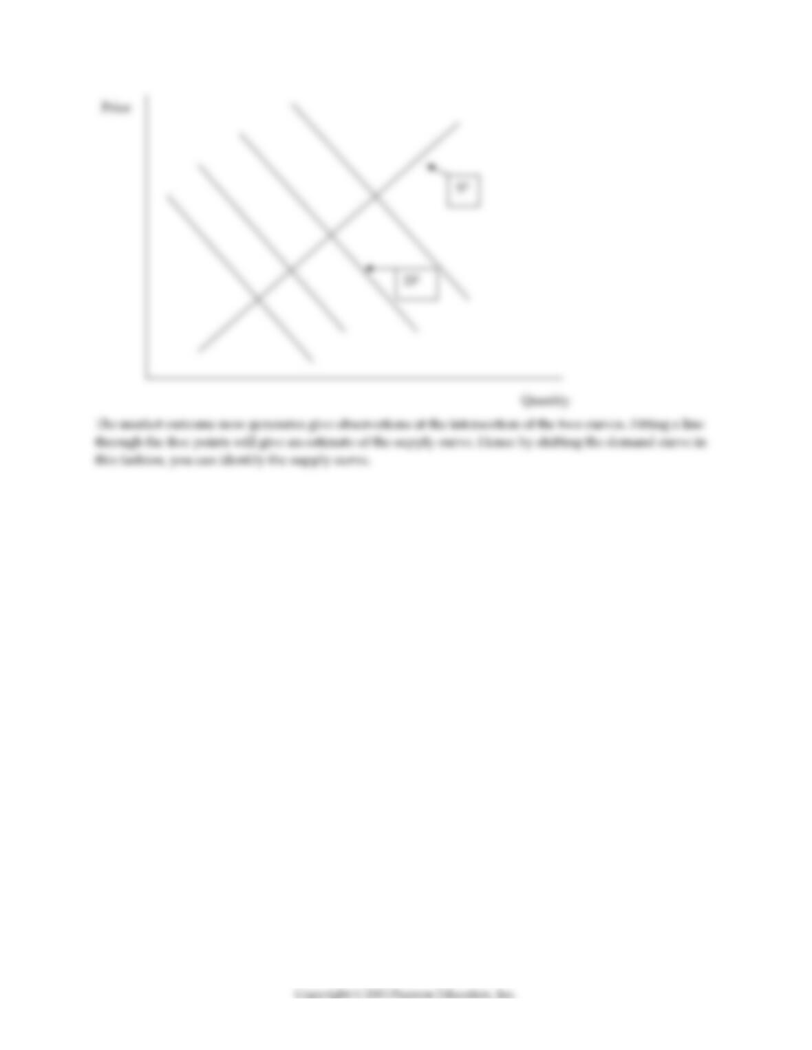
and explain why it is impossible to identify the demand and supply curves in such a situation. Next
assume that an additional variable enters the demand equation: income. In a new graph, draw the initial
position of the demand and supply curves and label them D0 and S0. Now allow for income to take on
four different values and sketch what happens to the two curves. Is there a pattern that you see which
suggests that you might be able to identify one of the two equations with real–life data?
31
17) Give at least three examples where you could envision errors–in–variables problems. For the case
where the measurement error occurs only for the explanatory variable in the simple regression case,
derive
2
11
22
ˆpX
Xw
⎯⎯→ +
.
18) Your textbook states that correlation of the error term across observations “will not happen if the data
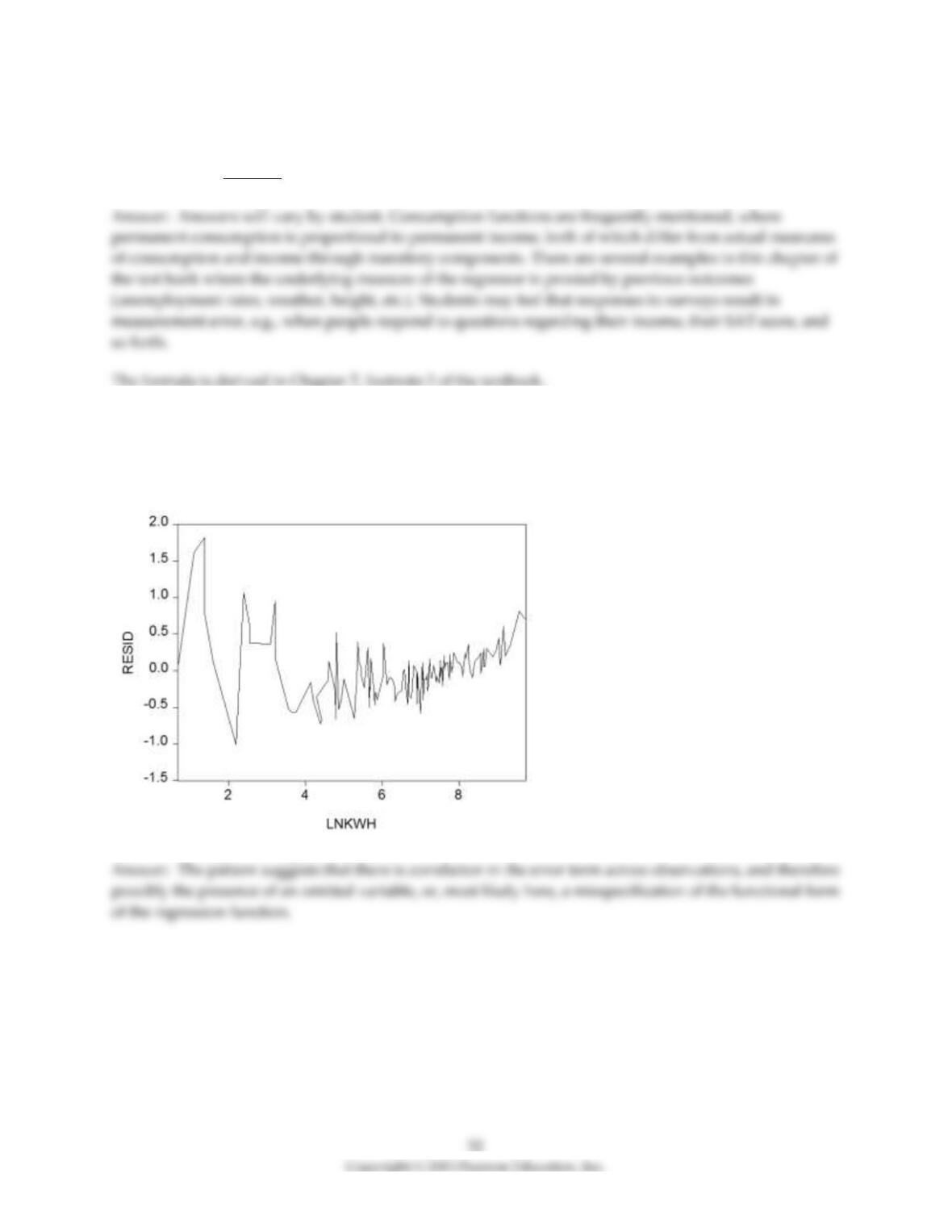
are obtained by sampling at random from the population.” However, in one famous study of the electric
utility industry, the observations were listed by the size of the output level, from smallest to largest. The
pattern of the residuals was as shown in the figure.
What does this pattern suggest to you?
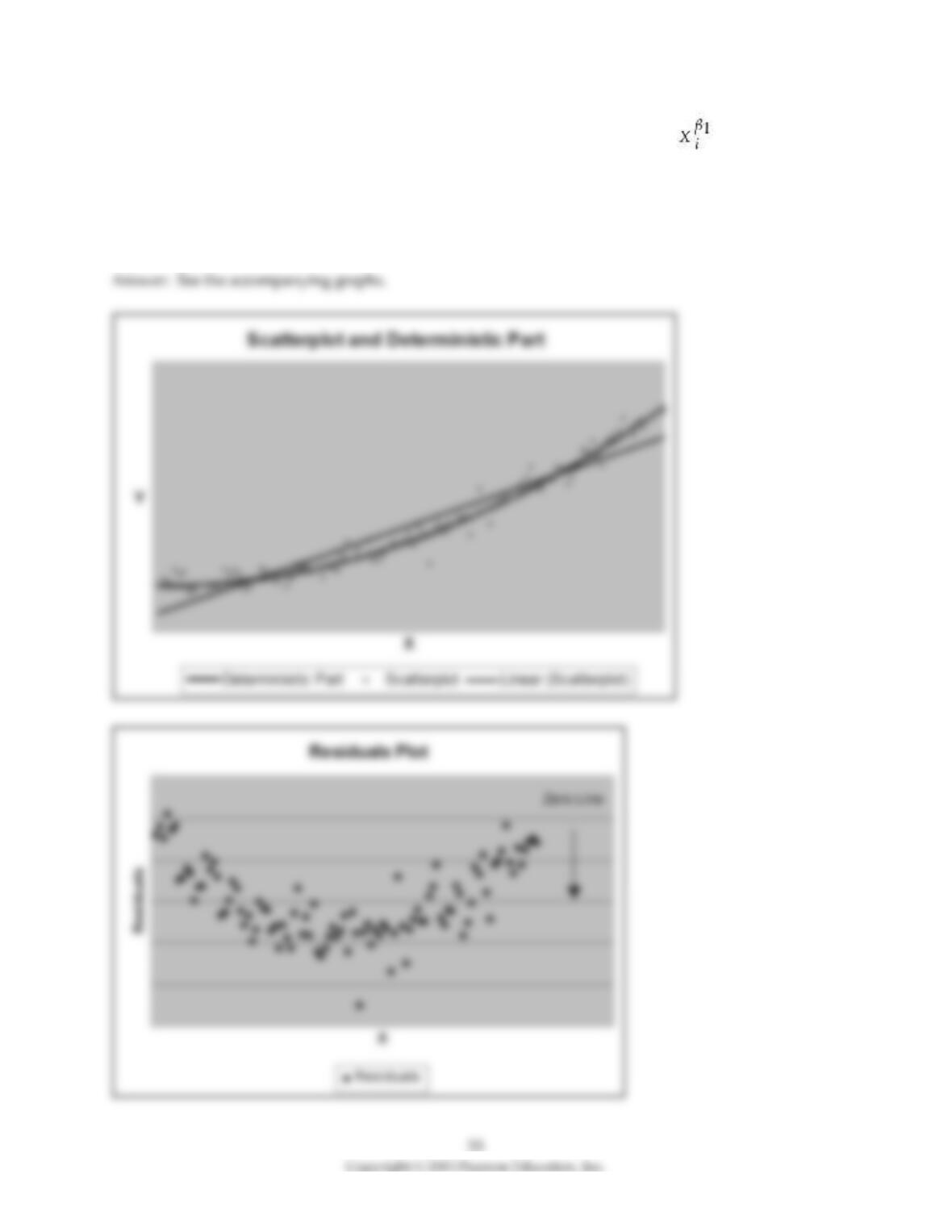
19) Consider a situation where Y is related to X in the following manner: Yi = β0 × × eui. Draw the
deterministic part of the above function. Next add, in the same graph, a hypothetical Y, X scatterplot of
the actual observations. Assume that you have misspecified the functional form of the regression function
and estimated the relationship between Y and X using a linear regression function. Add this linear
regression function to your graph. Separately, show what the plot of the residuals against the X variable
in your regression would look like.
34
20) In macroeconomics, you studied the equilibrium in the goods and money market under the
assumption of prices being fixed in the very short run. The goods market equilibrium was described by
the so–called IS equation
Ri = β0 – β1Yi + ui
where R represented the nominal interest rate and Y was real GDP. β0 contained variables determined
outside the system, such as government expenditures, taxes, and inflationary expectations.
The money market equilibrium was given by the so–called LM equation
Ri = + Yi + vi
and contained the real money supply and the intercept from the money demand equation.
Show that there is simultaneous causality bias in this situation.
21) Assume the following model of the labor market:
Nd = β0 + β1 + u
Ns = γ0 + γ1 + v
Nd = Ns = N
where N is employment, (W/P) is the real wage in the labor market, and u and v are determinants other
than the real wage which affect labor demand and labor supply (respectively). Let
E(u) = E(v) = 0; var(u) = ; var(v) = ; cov(u,v) = 0
Assume that you had collected data on employment and the real wage from a random sample of
observations and estimated a regression of employment on the real wage (employment being the
regressand and the real wage being the regressor). It is easy but tedious to show that
( )
( )
2
1 1 1 1 22
ˆpu
uv
− ⎯⎯→ − +
> 0
since the slope of the labor supply function is positive and the slope of the labor demand function is
negative. Hence, in general, you will not find the correct answer even in large samples.
a. What is this bias referred to?
b. What would the relationship between the variance of the labor supply/demand shift variable have to
be for the bias to disappear?
c. Give an intuitive answer why the bias would disappear in that situation. Draw a graph to illustrate
your argument.
36
22) To compare the slope coefficient from the California School data set with that of the Massachusetts
School data set, you run the following two regressions:
CA = 2.35 – 0.123×STRCA
(0.54) (0.027)
n = 420, R2 = 0.051, SER = 0.98
MA = 1.97 – 0.114×STRMA
(0.57) (0.033)
n = 220, R2 = 0.067, SER = 0.97
Numbers in parenthesis are heteroskedasticity–robust standard errors, and the LHS variable has been
standardized.
Calculate a t–statistic to test whether or not the two coefficients are the same. State the alternative
hypothesis. Which level of significance did you choose?
23) You have read the analysis in chapter 9 and want to explore the relationship between poverty and test
scores. You decide to start your analysis by running a regression of test scores on the percent of students
who are eligible to receive a free/reduced price lunch both in California and in Massachusetts. The results
are as follows:
CA = 681.44 – 0.610×PctLchCA
(0.99) (0.018)
n = 420, R2 = 0.75, SER = 9.45
MA = 731.89 – 0.788×PctLchMA
(0.95) (0.045)
n = 220, R2 = 0.61, SER = 9.41
Numbers in parenthesis are heteroskedasticity–robust standard errors.
a. Calculate a t–statistic to test whether or not the two slope coefficients are the same.
b. Your textbook compares the slope coefficients for the student–teacher ratio instead of the percent
eligible for a free lunch. The authors remark: “Because the two standardized tests are different, the
coefficients themselves cannot be compared directly: One point on the Massachusetts test is not the same
as one point on the California test.” What solution do they suggest?