11) You have collected 14,925 observations from the Current Population Survey. There are 6,285 females
in the sample, and 8,640 males. The females report a mean of average hourly earnings of $16.50 with a
standard deviation of $9.06. The males have an average of $20.09 and a standard deviation of $10.85. The
overall mean average hourly earnings is $18.58.
a. Using the t–statistic for testing differences between two means (section 3.4 of your textbook), decide
whether or not there is sufficient evidence to reject the null hypothesis that females and males have
identical average hourly earnings.
b. You decide to run two regressions: first, you simply regress average hourly earnings on an intercept
only. Next, you repeat this regression, but only for the 6,285 females in the sample. What will the
regression coefficients be in each of the two regressions?
c. Finally you run a regression over the entire sample of average hourly earnings on an intercept and a
binary variable DFemme, where this variable takes on a value of 1 if the individual is a female, and is 0
otherwise. What will be the value of the intercept? What will be the value of the coefficient of the binary
variable?
d. What is the standard error on the slope coefficient? What is the t–statistic?
e. Had you used the homoskedasticity–only standard error in (d) and calculated the t–statistic, how would
you have had to change the test–statistic in (a) to get the identical result?
5.3 Mathematical and Graphical Problems
1) In order to formulate whether or not the alternative hypothesis is one–sided or two–sided, you need
some guidance from economic theory. Choose at least three examples from economics or other fields
where you have a clear idea what the null hypothesis and the alternative hypothesis for the slope
coefficient should be. Write a brief justification for your answer.
2) For the following estimated slope coefficients and their heteroskedasticity robust standard errors, find
the t–statistics for the null hypothesis H0: β1 = 0. Assuming that your sample has more than 100
observations, indicate whether or not you are able to reject the null hypothesis at the 10%, 5%, and 1%
level of a one–sided and two–sided hypothesis.
(a) 1 = 4.2, SE(1) = 2.4
(b) 1 = 0.5, SE(1) = 0.37
(c) 1 = 0.003, SE(1) = 0.002
(d) 1 = 360, SE(1) = 300
3) Explain carefully the relationship between a confidence interval, a one–sided hypothesis test, and a
two–sided hypothesis test. What is the unit of measurement of the t–statistic?
4) The effect of decreasing the student–teacher ratio by one is estimated to result in an improvement of the
districtwide score by 2.28 with a standard error of 0.52. Construct a 90% and 99% confidence interval for
the size of the slope coefficient and the corresponding predicted effect of changing the student–teacher
ratio by one. What is the intuition on why the 99% confidence interval is wider than the 90% confidence
interval?
5) Below you are asked to decide on whether or not to use a one–sided alternative or a two–sided
alternative hypothesis for the slope coefficient. Briefly justify your decision.
(a)
ˆd
i
q
= 0 + 1pi, where qd is the quantity demanded for a good, and p is its price.
(b)
ˆactual
i
p
= 0 + 1
ˆactual
i
p
, where
ˆactual
i
p
is the actual house price, and
ˆactual
i
p
is the assessed house price.
You want to test whether or not the assessment is correct, on average.
(c) i = 0 + 1
d
i
Y
, where C is household consumption, and Yd is personal disposable income.
6) (Requires Appendix material) Your textbook shows that OLS is a linear estimator 1 =
1
ˆ
n
ii
i
aY
=
, where
( )
2
1
ˆi
in
i
i
XX
a
XX
=
−
=
−
. For OLS to be conditionally unbiased, the following two conditions must hold:
1
ˆ0
n
i
i
a
=
=
and
1
ˆ
n
ii
i
aX
=
= 1. Show that this is the case.
7) (Requires Appendix material and Calculus) Equation (5.36) in your textbook derives the conditional
variance for any old conditionally unbiased estimator 1 to be var( 1X1, …, Xn) =
22
1
n
ui
i
a
=
where the
conditions for conditional unbiasedness are
1
n
i
i
a
=
= 0 and
1
n
ii
i
aX
=
= 1. As an alternative to the BLUE
proof presented in your textbook, you recall from one of your calculus courses that you could minimize
the variance subject to the two constraints, thereby making the variance as small as possible while the
constraints are holding. Show that in doing so you get the OLS weights
ˆi
a
. (You may assume that X1,…,
Xn are nonrandom (fixed over repeated samples).)
8) Your textbook states that under certain restrictive conditions, the t– statistic has a Student t–distribution
with n–2 degrees of freedom. The loss of two degrees of freedom is the result of OLS forcing two
restrictions onto the data. What are these two conditions, and when did you impose them onto the data
set in your derivation of the OLS estimator?
n
n
9) Assume that your population regression function is
Yi = βiXi + ui
i.e., a regression through the origin (no intercept). Under the homoskedastic normal regression
assumptions, the t–statistic will have a Student t distribution with n–1 degrees of freedom, not n–2 degrees
of freedom, as was the case in Chapter 5 of your textbook. Explain. Do you think that the residuals will
still sum to zero for this case?
n
10) In many of the cases discussed in your textbook, you test for the significance of the slope at the 5%
level. What is the size of the test? What is the power of the test? Why is the probability of committing a
Type II error so large here?
11) Assume that the homoskedastic normal regression assumption hold. Using the Student t–distribution,
find the critical value for the following situation:
(a) n = 28, 5% significance level, one–sided test.
(b) n = 40, 1% significance level, two–sided test.
(c) n = 10, 10% significance level, one–sided test.
(d) n = ∞, 5% significance level, two–sided test.
22
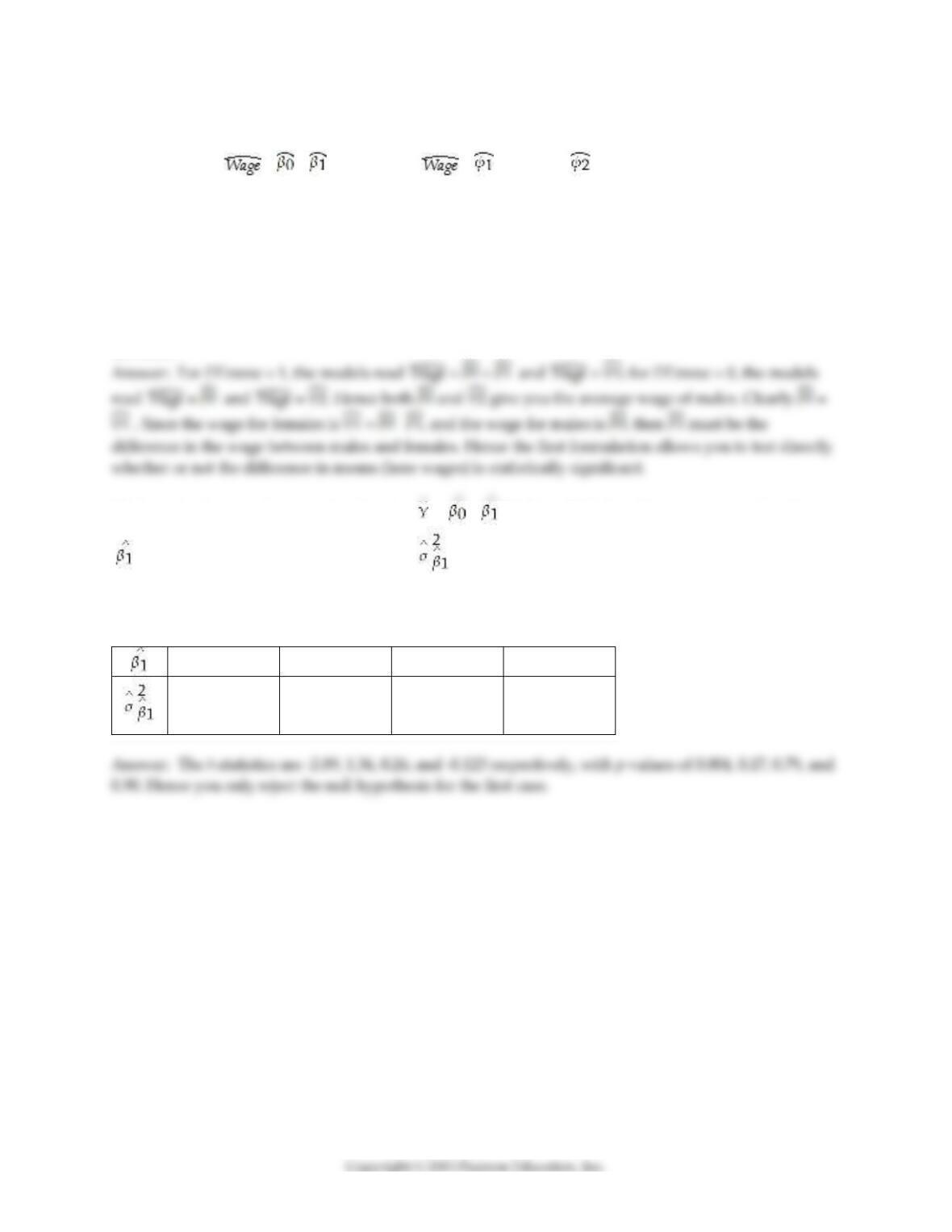
12) Consider the following two models involving binary variables as explanatory variables:
= + DFemme and = DFemme + Male
where Wage is the hourly wage rate, DFemme is a binary variable that is equal to 1 if the person is a
female, and 0 if the person is a male. Male = 1 – DFemme. Even though you have not learned about
regression functions with two explanatory variables (or regressions without an intercept), assume that
you had estimated both models, i.e., you obtained the estimates for the regression coefficients.
What is the predicted wage for a male in the two models? What is the predicted wage for a female in the
two models? What is the relationship between the β s and the φs? Why would you prefer one model over
the other?
13) Consider the sample regression function i = + Xi. The table below lists estimates for the slope
() and the variance of the slope estimator ( ). In each case calculate the p–value for the null
hypothesis of β1 = 0 and a two–tailed alternative hypothesis. Indicate in which case you would reject the
null hypothesis at the 5% significance level.
–1.76
0.0025
2.85
–0.00014
0.37
0.000003
117.5
0.0000013
14) Your textbook discussed the regression model when X is a binary variable
Yi = β0 + β1Di + ui, i = 1…, n
Let Y represent wages, and let D be one for females, and 0 for males. Using the OLS formula for the slope
coefficient, prove that is the difference between the average wage for males and the average wage for
females.
15) Your textbook discussed the regression model when X is a binary variable
Yi = β0 + βiDi + ui, i = 1,…, n
Let Y represent wages, and let D be one for females, and 0 for males. Using the OLS formula for the
intercept coefficient, prove that is the average wage for males.
16) Let
i
u
be distributed N(0,
2
u
), i.e., the errors are distributed normally with a constant variance
(homoskedasticity). This results in being distributed N(β1,
2
ˆ1
), where
( )
2
2
ˆ12
1
u
n
i
i
XX
=
=
−
. Statistical
inference would be straightforward if
2
u
was known. One way to deal with this problem is to replace
2
u
with an estimator
2
ˆ
u
S
. Clearly since this introduces more uncertainty, you cannot expect to be still
normally distributed. Indeed, the t–statistic now follows Student’s t distribution. Look at the table for the
Student t–distribution and focus on the 5% two–sided significance level. List the critical values for 10
degrees of freedom, 30 degrees of freedom, 60 degrees of freedom, and finally ∞ degrees of freedom.
Describe how the notion of uncertainty about
2
u
can be incorporated about the tails of the t–distribution
as the degrees of freedom increase.
2
ˆ
u
S
2
u

25
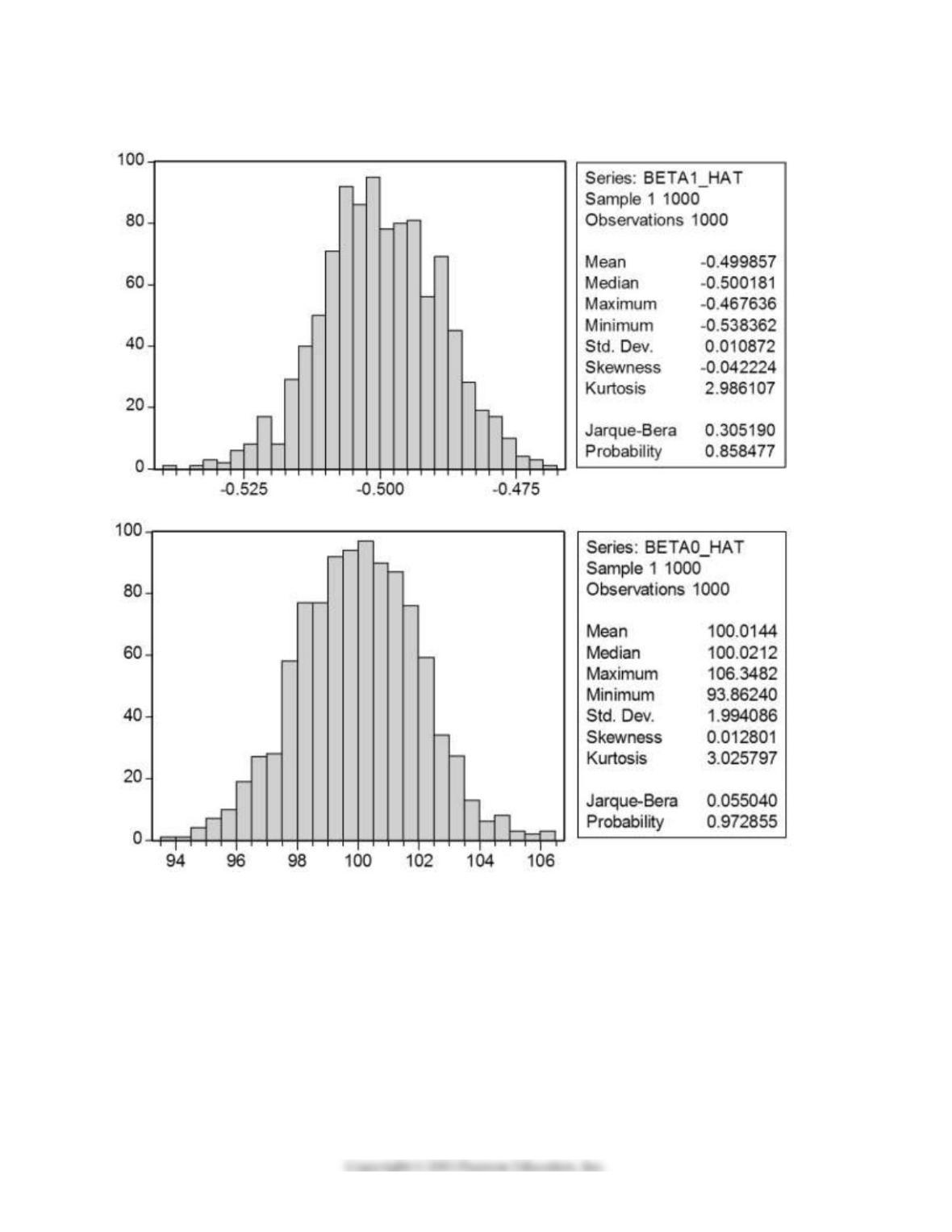
17) In a Monte Carlo study, econometricians generate multiple sample regression functions from a known
population regression function. For example, the population regression function could be Yi = β0 + β1Xi =
100 – 0.5 Xi. The Xs could be generated randomly or, for simplicity, be nonrandom (“fixed over repeated
samples”). If we had ten of these Xs, say, and generated twenty Ys, we would obviously always have all
observations on a straight line, and the least squares formulae would always return values of 100 and 0.5
numerically. However, if we added an error term, where the errors would be drawn randomly from a
normal distribution, say, then the OLS formulae would give us estimates that differed from the
population regression function values. Assume you did just that and recorded the values for the slope
and the intercept. Then you did the same experiment again (each one of these is called a “replication”).
And so forth. After 1,000 replications, you plot the 1,000 intercepts and slopes, and list their summary
statistics.
Sample: 1 1000
BETA0_HAT BETA1_HAT
Mean 100.014 –0.500
Median 100.021 –0.500
Maximum 106.348 –0.468
Minimum 93.862 –0.538
Std. Dev. 1.994 0.011
Skewness 0.013 –0.042
Kurtosis 3.026 2.986
Jarque–Bera 0.055 0.305
Probability 0.973 0.858
Sum 100014.353 –499.857
Sum Sq. Dev. 3972.403 0.118
Observations 1000.000 1000.000
26
Here are the corresponding graphs:
Using the means listed next to the graphs, you see that the averages are not exactly 100 and –0.5.
However, they are “close.” Test for the difference of these averages from the population values to be
statistically significant.
27
18) In the regression through the origin model Yi = β1Xi + ui, the OLS estimator is 1 =
1
2
1
n
ii
i
n
i
i
XY
X
=
=
. Prove
that the estimator is a linear function of Y1,…, Yn and prove that it is conditionally unbiased.
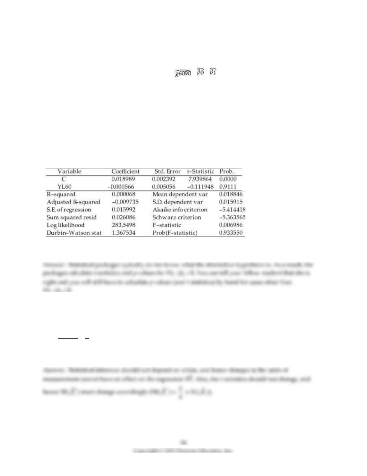
19) The neoclassical growth model predicts that for identical savings rates and population growth rates,
countries should converge to the per capita income level. This is referred to as the convergence
hypothesis. One way to test for the presence of convergence is to compare the growth rates over time to
the initial starting level, i.e., to run the regression = + × RelProd60 , where g6090 is the
average annual growth rate of GDP per worker for the 1960–1990 sample period, and RelProd60 is GDP
per worker relative to the United States in 1960. Under the null hypothesis of no convergence, β1 = 0; H1 :
β1 < 0, implying (“beta”) convergence. Using a standard regression package, you get the following output:
Dependent Variable: G6090
Method: Least Squares
Date: 07/11/06 Time: 05:46
Sample: 1 104
Included observations: 104
White Heteroskedasticity–Consistent Standard Errors & Covariance
You are delighted to see that this program has already calculated p–values for you. However, a peer of
yours points out that the correct p–value should be 0.4562. Who is right?
20) Changing the units of measurement obviously will have an effect on the slope of your regression
function. For example, let Y*= aY and X* = bX. Then it is easy but tedious to show that
1
11
2
1
ˆˆ
n
ii
i
n
i
i
xy a
b
x
=
=
==
. Given this result, how do you think the standard errors and the regression R2 will
change?
21) Using the California School data set from your textbook, you run the following regression:
= 698.9 – 2.28 STR
n = 420, SER = 9.4
where TestScore is the average test score in the district and STR is the student–teacher ratio. The sample
standard deviation of test scores is 19.05, and the sample standard deviation of the student teacher ratio is
1.89.
a.
Find the regression R2 and the correlation coefficient between test scores and the student teacher ratio.
b.
Find the homoskedasticity–only standard error of the slope.
22) Using the California School data set from your textbook, you run the following regression:
= 698.9 – 2.28 STR
n = 420, R2 = 0.051, SER = 18.6
where TestScore is the average test score in the district and STR is the student-teacher ratio. Using
heteroskedasticity robust standard errors, you find
while choosing the homoskedasticity-only option, the standard error is 0.48.
a. Calculate the t-statistic for both standard errors.
b. Which of the two t-statistics should you base your inference on?
23) Using data from the Current Population Survey, you estimate the following relationship between
average hourly earnings (ahe) and the number of years of education (educ):
= -4.58 + 1.71 educ
The heteroskedasticity-robust standard error on the slope is (0.03). Calculate the 95% confidence interval
for the slope. Repeat the exercise using the 90% and then the 99% confidence interval. Can you reject the
null hypothesis that the slope coefficient is zero in the population?