10) During the last few days before a presidential election, there is a frenzy of voting intention surveys.
On a given day, quite often there are conflicting results from three major polls.
(a) Think of each of these polls as reporting the fraction of successes (1s) of a Bernoulli random variable Y,
where the probability of success is Pr(Y = 1) = p. Let
ˆ
p
be the fraction of successes in the sample and
assume that this estimator is normally distributed with a mean of p and a variance of
( )
1pp
n
−
. Why are
the results for all polls different, even though they are taken on the same day?
(b) Given the estimator of the variance of
ˆ
p
,
( )
ˆˆ
1pp
n
−
, construct a 95% confidence interval for
ˆ
p
. For
which value of
ˆ
p
is the standard deviation the largest? What value does it take in the case of a maximum
ˆ
p
?
(c) When the results from the polls are reported, you are told, typically in the small print, that the “margin
of error” is plus or minus two percentage points. Using the approximation of 1.96 ≈ 2, and assuming,
“conservatively,” the maximum standard deviation derived in (b), what sample size is required to add
and subtract (“margin of error”) two percentage points from the point estimate?
(d) What sample size would you need to halve the margin of error?
ˆ
p
ˆ
p
ˆ
p
11) At the Stock and Watson (http://www.pearsonhighered.com/stock_watson) website go to Student
Resources and select the option “Datasets for Replicating Empirical Results.” Then select the “CPS Data
Used in Chapter 8″ (ch8_cps.xls) and open it in Excel. This is a rather large data set to work with, so just
copy the first 500 observations into a new Worksheet (these are rows 1 to 501).
In the newly created Worksheet, mark A1 to A501, then select the Data tab and click on “sort.” A dialog
box will open. First select “Add level” from one of the options on the left. Then select “sort by” and choose
“Northeast” and “Largest to Smallest.” Repeat the same for the “South” as a second option. Finally press
“ok.”
This should give you 209 observations for average hourly earnings for the Northeast region, followed by
205 observations for the South.
a. For each of the 209 average hourly earnings observations for the Northeast region and separately for
the South region, calculate the mean and sample standard deviation.
b Use the appropriate test to determine whether or not average hourly earnings in the Northeast region
the same as in the South region.
c Find the 1%, 5%, and 10% confidence interval for the differences between the two population means.
Is your conclusion consistent with the test in part (b)?
d In all three cases of using the confidence interval in (c), the power of the test is quite low (5%). What
can you do to increase the power of the test without reducing the size of the test?
19
3.3 Mathematical and Graphical Problems
1) Your textbook defined the covariance between X and Y as follows:
( )( )
1
1
1
n
ii
i
X X Y Y
n=
−−
−
Prove that this is identical to the following alternative specification:
1
1
11
n
ii
i
n
X Y XY
nn
=
−
−−
20
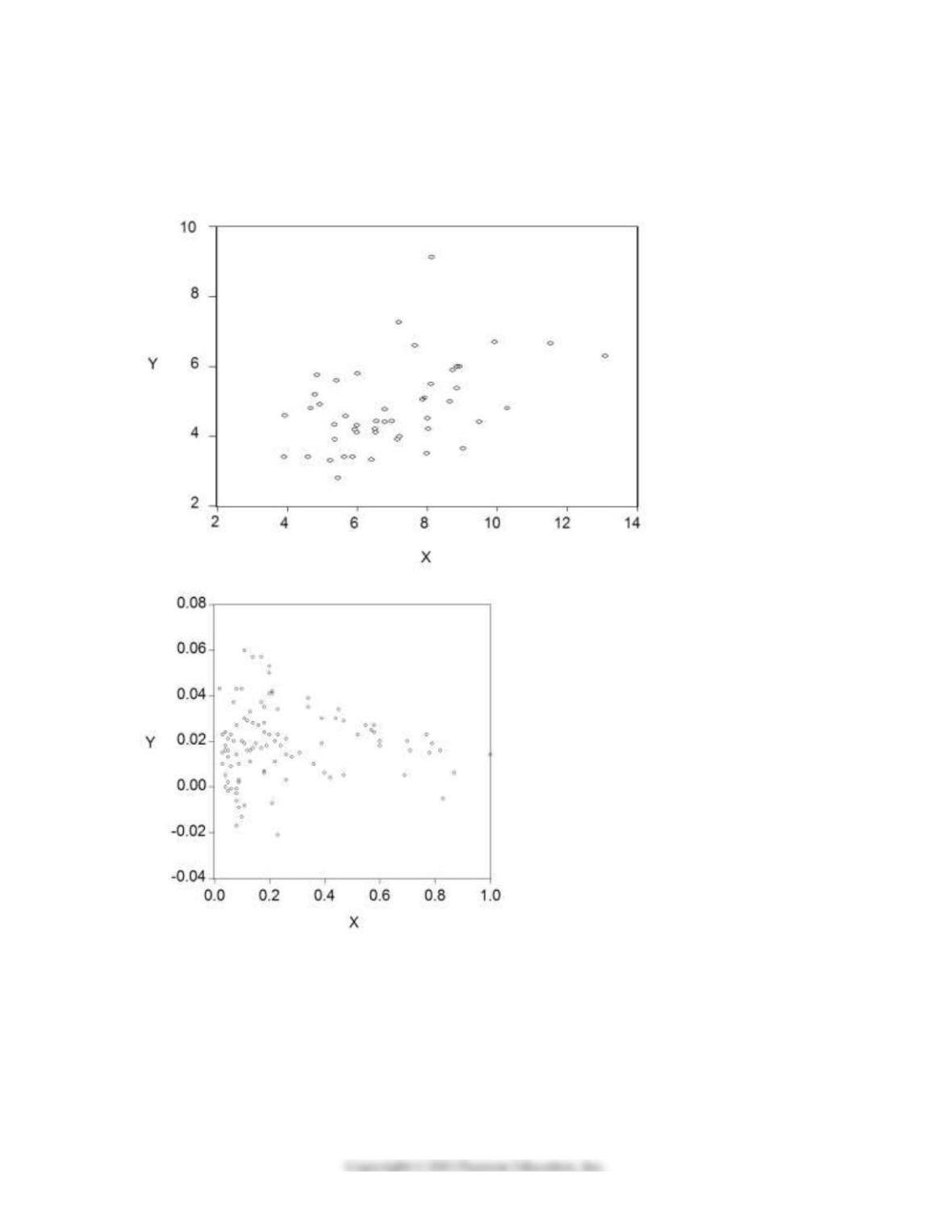
2) For each of the accompanying scatterplots for several pairs of variables, indicate whether you expect a
positive or negative correlation coefficient between the two variables, and the likely magnitude of it (you
can use a small range).
(a)
(b)
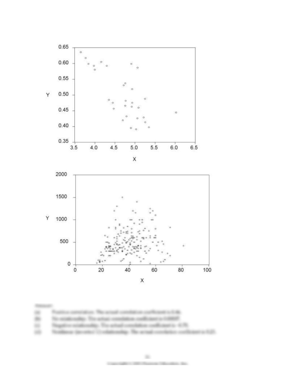
(c)
(d)
22
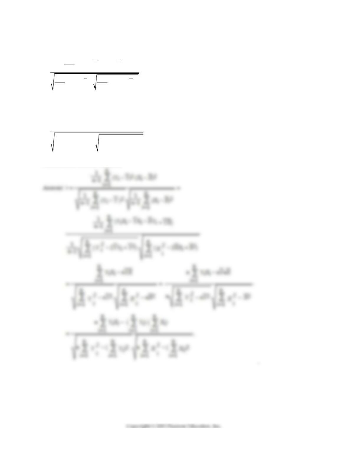
3) Your textbook defines the correlation coefficient as follows:
( ) ( )
( ) ( )
22
1
22
11
1
1
11
11
n
ii
i
nn
ii
ii
Y Y X X
n
r
Y Y X X
nn
=
==
−−
−
=
−−
−−
Another textbook gives an alternative formula:
1 1 1
22
22
1 1 1 1
n n n
i i i i
i i i
n n n n
i i i i
i i i i
n Y X Y X
r
n Y Y n X X
= = =
= = = =
−
=
−−
Prove that the two are the same.
23
4) IQs of individuals are normally distributed with a mean of 100 and a standard deviation of 16. If you
sampled students at your college and assumed, as the null hypothesis, that they had the same IQ as the
population, then in a random sample of size
(a) n = 25, find Pr(
Y
< 105).
(b) n = 100, find Pr(
Y
> 97).
(c) n = 144, find Pr(101 <
Y
< 103).
Answer:
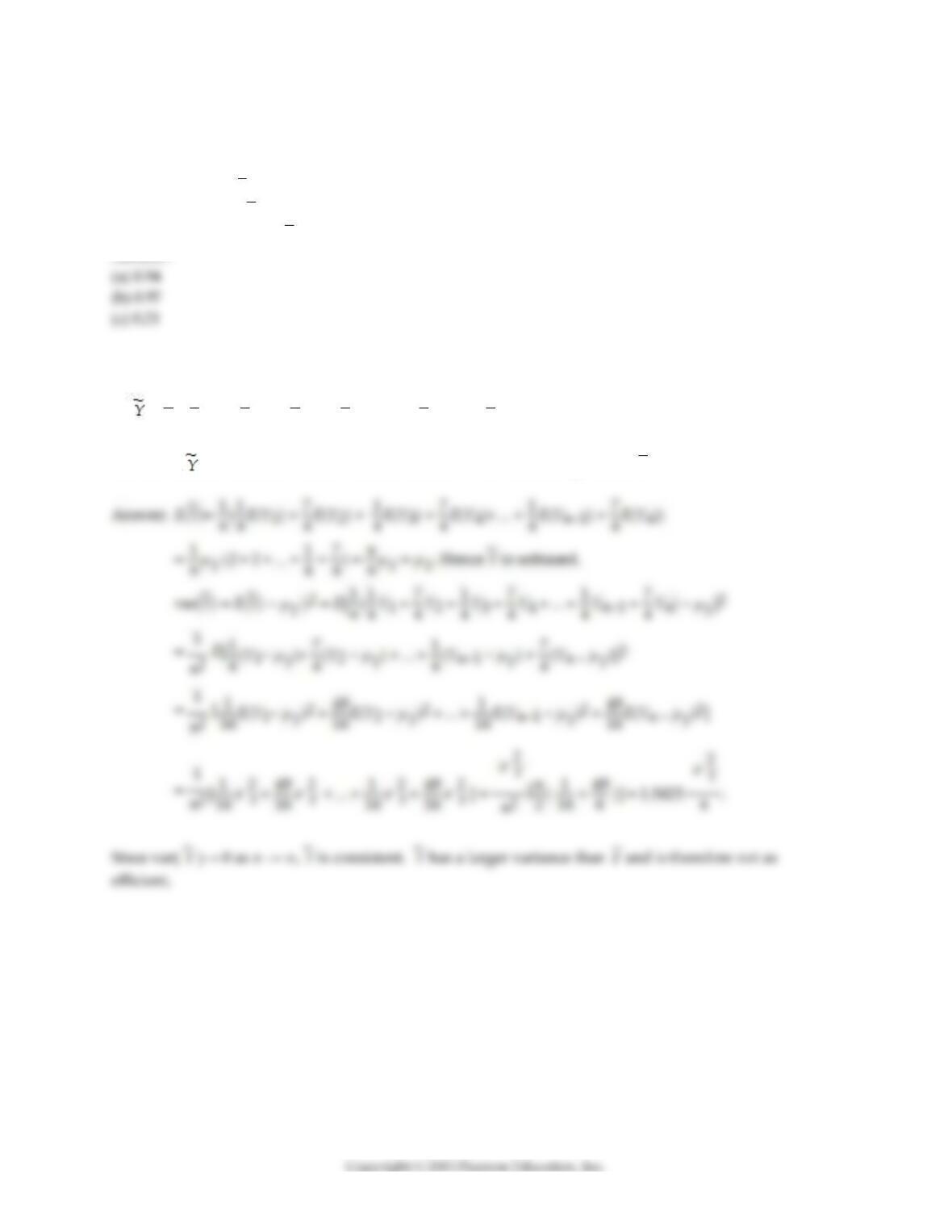
5) Consider the following alternative estimator for the population mean:
=
1
n
(
1
4
Y1 +
7
4
Y2 +
1
4
Y3 +
7
4
Y4 + … +
1
4
Yn–1 +
7
4
Yn)
Prove that is unbiased and consistent, but not efficient when compared to
Y
.
Y
6) Imagine that you had sampled 1,000,000 females and 1,000,000 males to test whether or not females
have a higher IQ than males. IQs are normally distributed with a mean of 100 and a standard deviation of
16. You are excited to find that females have an average IQ of 101 in your sample, while males have an IQ
of 99. Does this difference seem important? Do you really need to carry out a t–test for differences in
means to determine whether or not this difference is statistically significant? What does this result tell
you about testing hypotheses when sample sizes are very large?
7) Let Y be a Bernoulli random variable with success probability Pr(Y = 1) = p, and let Y1,…, Yn be i.i.d.
draws from this distribution. Let
ˆ
p
be the fraction of successes (1s) in this sample. In large samples, the
distribution of
ˆ
p
will be approximately normal, i.e.,
ˆ
p
is approximately distributed N(p,
( )
1pp
n
−
). Now
let X be the number of successes and n the sample size. In a sample of 10 voters (n=10), if there are six who
vote for candidate A, then X = 6. Relate X, the number of success, to
ˆ
p
, the success proportion, or fraction
of successes. Next, using your knowledge of linear transformations, derive the distribution of X.
ˆ
p
ˆ
p
ˆ
p
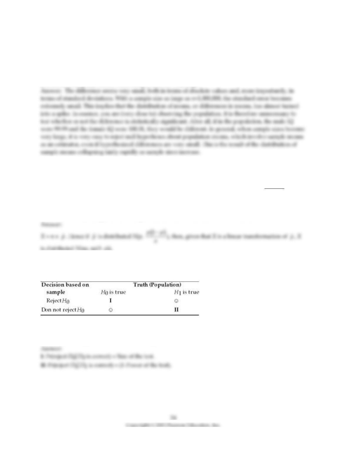
8) When you perform hypothesis tests, you are faced with four possible outcomes described in the
accompanying table.
“☺” indicates a correct decision, and I and II indicate that an error has been made. In probability terms,
state the mistakes that have been made in situation I and II, and relate these to the Size of the test and the
Power of the test (or transformations of these).
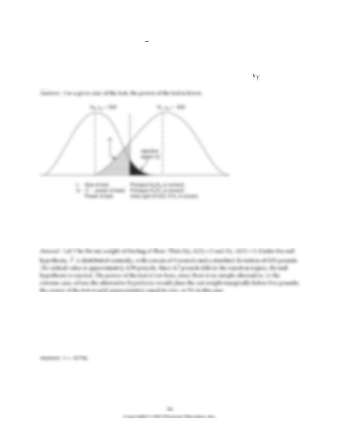
9) Assume that under the null hypothesis,
Y
has an expected value of 500 and a standard deviation of 20.
Under the alternative hypothesis, the expected value is 550. Sketch the probability density function for
the null and the alternative hypothesis in the same figure. Pick a critical value such that the p–value is
approximately 5%. Mark the areas, which show the size and the power of the test. What happens to the
power of the test if the alternative hypothesis moves closer to the null hypothesis, i.e.,, = 540, 530, 520,
etc.?
10) The net weight of a bag of flour is guaranteed to be 5 pounds with a standard deviation of 0.05
pounds. You are concerned that the actual weight is less. To test for this, you sample 25 bags. Carefully
state the null and alternative hypothesis in this situation. Determine a critical value such that the size of
the test does not exceed 5%. Finding the average weight of the 25 bags to be 4.7 pounds, can you reject the
null hypothesis? What is the power of the test here? Why is it so low?
11) Some policy advisors have argued that education should be subsidized in developing countries to
reduce fertility rates. To investigate whether or not education and fertility are correlated, you collect data
on population growth rates (Y) and education (X) for 86 countries. Given the sums below, compute the
sample correlation:
1
n
i
i
Y
=
= 1.594;
1
n
i
i
X
=
= 449.6;
1
n
ii
i
YX
=
= 6.4697;
2
1
n
i
i
Y
=
= 0.03982;
2
1
n
i
i
X
=
= 3,022.76
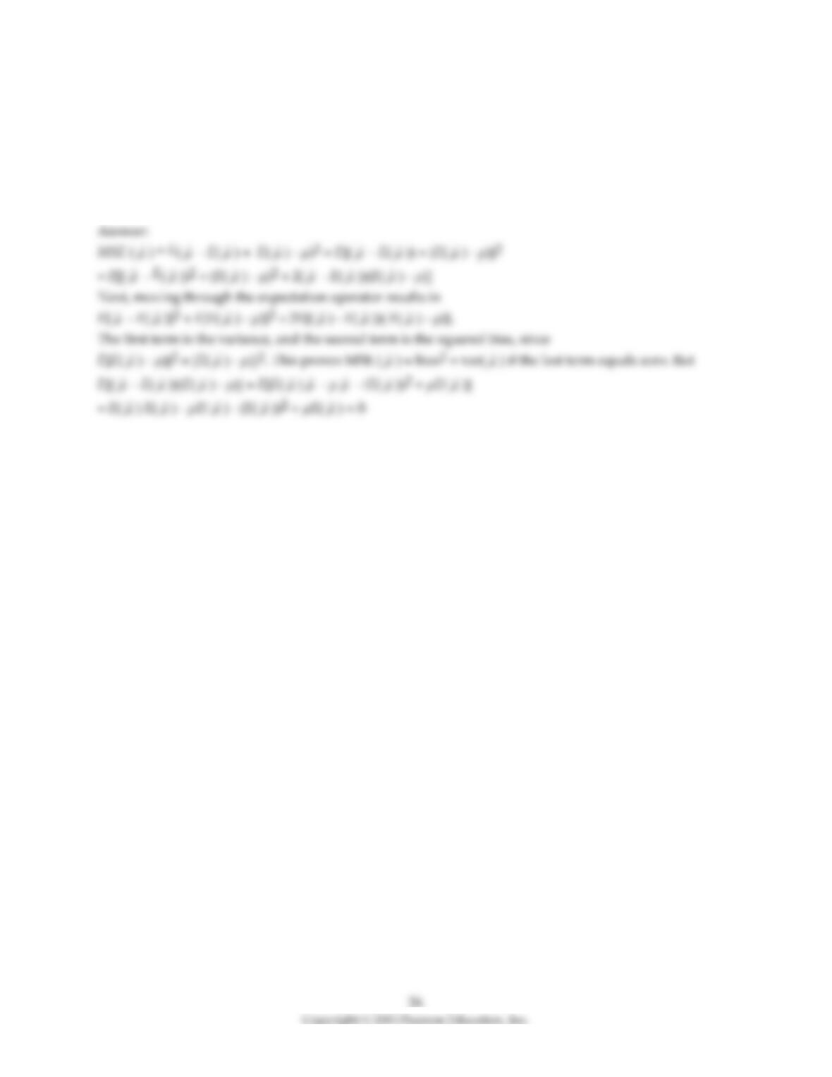
12) (Advanced) Unbiasedness and small variance are desirable properties of estimators. However, you
can imagine situations where a trade–off exists between the two: one estimator may be have a small bias
but a much smaller variance than another, unbiased estimator. The concept of “mean square error”
estimator combines the two concepts. Let
ˆ
be an estimator of μ. Then the mean square error (MSE) is
defined as follows: MSE(
ˆ
) = E(
ˆ
– μ)2. Prove that MSE(
ˆ
) = bias2 + var(
ˆ
). (Hint: subtract and add in
E(
ˆ
) in E(
ˆ
– μ)2.)
ˆ
ˆ
ˆ
ˆ
ˆ
ˆ
ˆ
ˆ
ˆ
ˆ
ˆ
ˆ
ˆ
ˆ
ˆ
ˆ
ˆ
ˆ
ˆ
ˆ
ˆ
ˆ
ˆ
ˆ
ˆ
ˆ
ˆ
ˆ
ˆ
ˆ
ˆ
ˆ
ˆ
ˆ
ˆ
ˆ
13) Your textbook states that when you test for differences in means and you assume that the two
population variances are equal, then an estimator of the population variance is the following “pooled”
estimator:
( ) ( )
22
2
11
1
2
mw
nn
w
pooled i m i
ii
mw
S Y Y Y Y
nn ==
= − + −
+−
Explain why this pooled estimator can be looked at as the weighted average of the two variances.
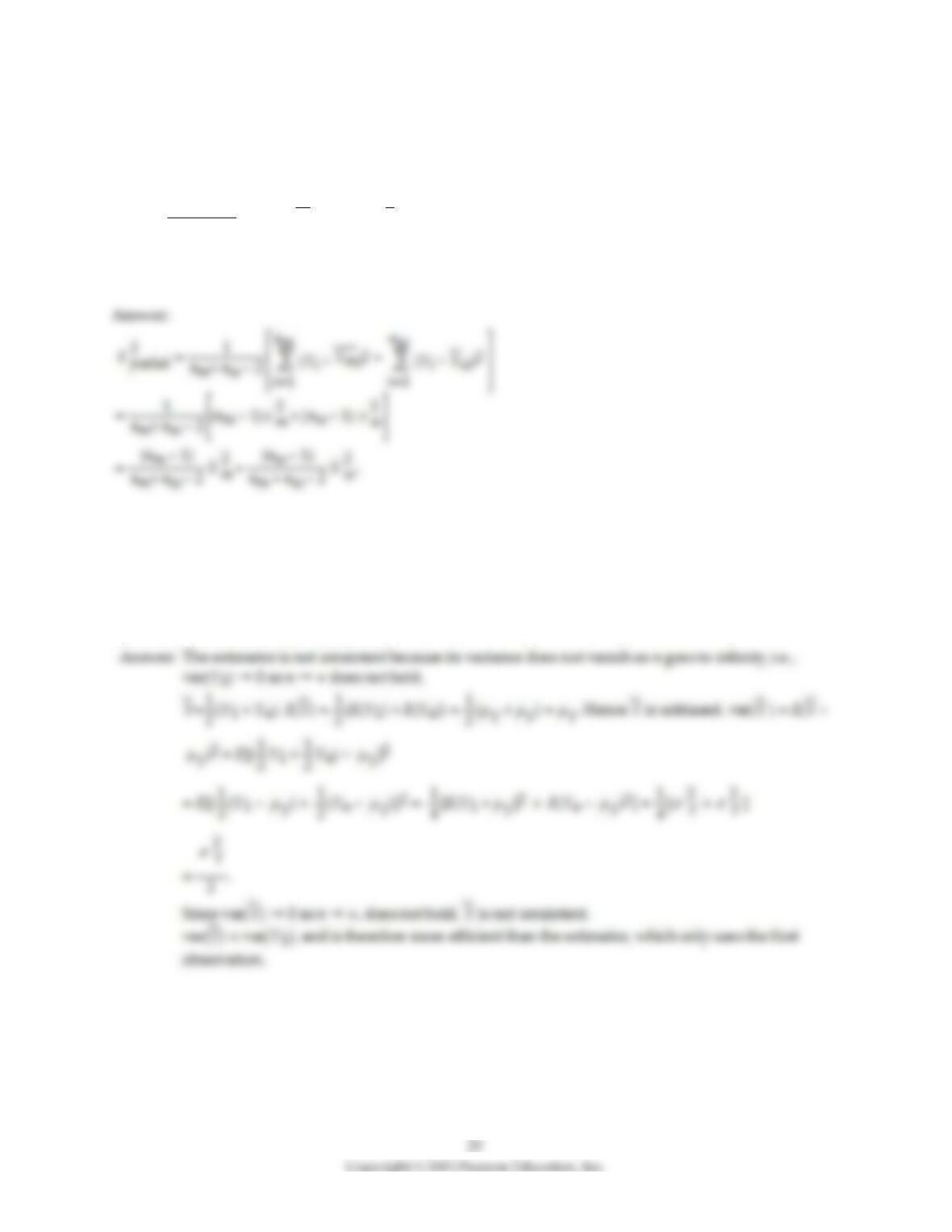
14) Your textbook suggests using the first observation from a sample of n as an estimator of the
population mean. It is shown that this estimator is unbiased but has a variance of
2
Y
, which makes it less
efficient than the sample mean. Explain why this estimator is not consistent. You develop another
estimator, which is the simple average of the first and last observation in your sample. Show that this
estimator is also unbiased and show that it is more efficient than the estimator which only uses the first
observation. Is this estimator consistent?
28
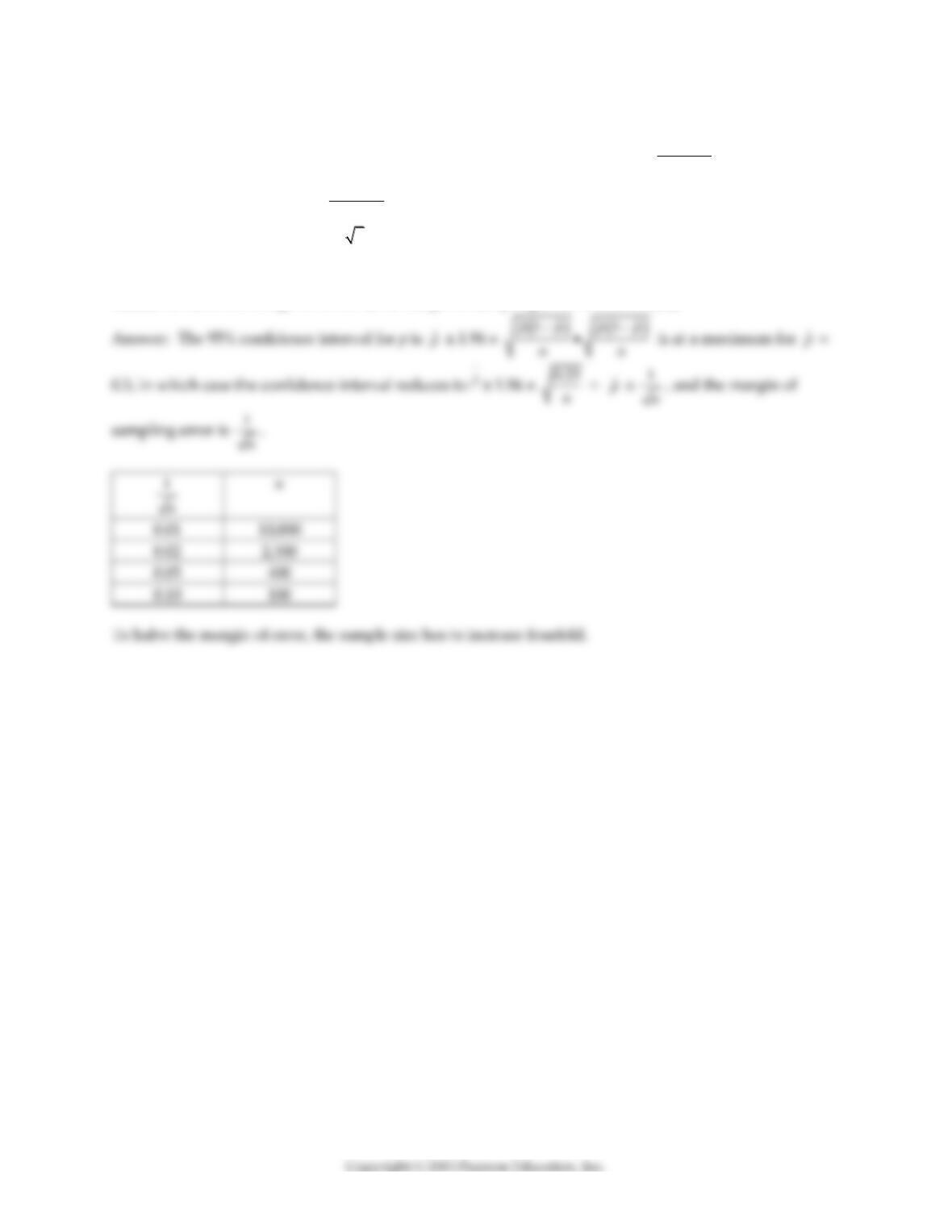
15) Let p be the success probability of a Bernoulli random variable Y, i.e., p = Pr(Y = 1). It can be shown
that
ˆ
p
, the fraction of successes in a sample, is asymptotically distributed N(p,
( )
1pp
n
−
. Using the
estimator of the variance of
ˆ
p
,
( )
ˆˆ
1pp
n
−
, construct a 95% confidence interval for p. Show that the margin
for sampling error simplifies to 1/
n
if you used 2 instead of 1.96 assuming, conservatively, that the
standard error is at its maximum. Construct a table indicating the sample size needed to generate a
margin of sampling error of 1%, 2%, 5% and 10%. What do you notice about the increase in sample size
needed to halve the margin of error? (The margin of sampling error is 1.96×SE(
ˆ
p
))
ˆ
p
ˆ
p
ˆ
p
16) Let Y be a Bernoulli random variable with success probability Pr(Y = 1) = p, and let Y1 ,…, Yn be i.i.d.
draws from this distribution. Let
ˆ
p
be the fraction of successes (1s) in this sample. Given the following
statement
Pr(–1.96 < z < 1.96) = 0.95
and assuming that
ˆ
p
being approximately distributed N(p,
( )
1pp
n
−
, derive the 95% confidence interval
for p by solving the above inequalities.
17) Your textbook mentions that dividing the sample variance by n –1 instead of n is called a degrees of
freedom correction. The meaning of the term stems from the fact that one degree of freedom is used up
when the mean is estimated. Hence degrees of freedom can be viewed as the number of independent
observations remaining after estimating the sample mean.
Consider an example where initially you have 20 independent observations on the height of students.
After calculating the average height, your instructor claims that you can figure out the height of the 20th
student if she provides you with the height of the other 19 students and the sample mean. Hence you
have lost one degree of freedom, or there are only 19 independent bits of information. Explain how you
can find the height of the 20th student.
18) The accompanying table lists the height (STUDHGHT) in inches and weight (WEIGHT) in pounds of
five college students. Calculate the correlation coefficient.
STUDHGHT WEIGHT
74 165
73 165
72 145
68 155
66 140
30
19) (Requires calculus.) Let Y be a Bernoulli random variable with success probability Pr(Y = 1) = p. It can
be shown that the variance of the success probability p is
( )
1pp
n
−
. Use calculus to show that this
variance is maximized for p = 0.5.
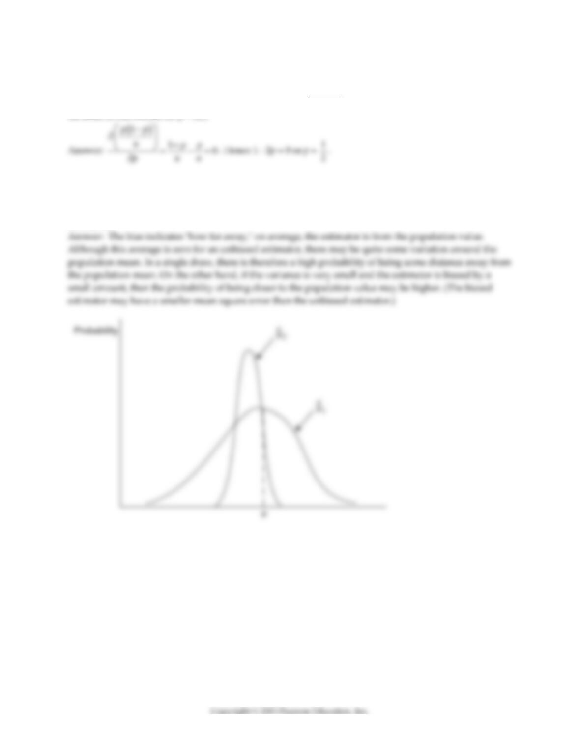
20) Consider two estimators: one which is biased and has a smaller variance, the other which is unbiased
and has a larger variance. Sketch the sampling distributions and the location of the population parameter
for this situation. Discuss conditions under which you may prefer to use the first estimator over the
second one.
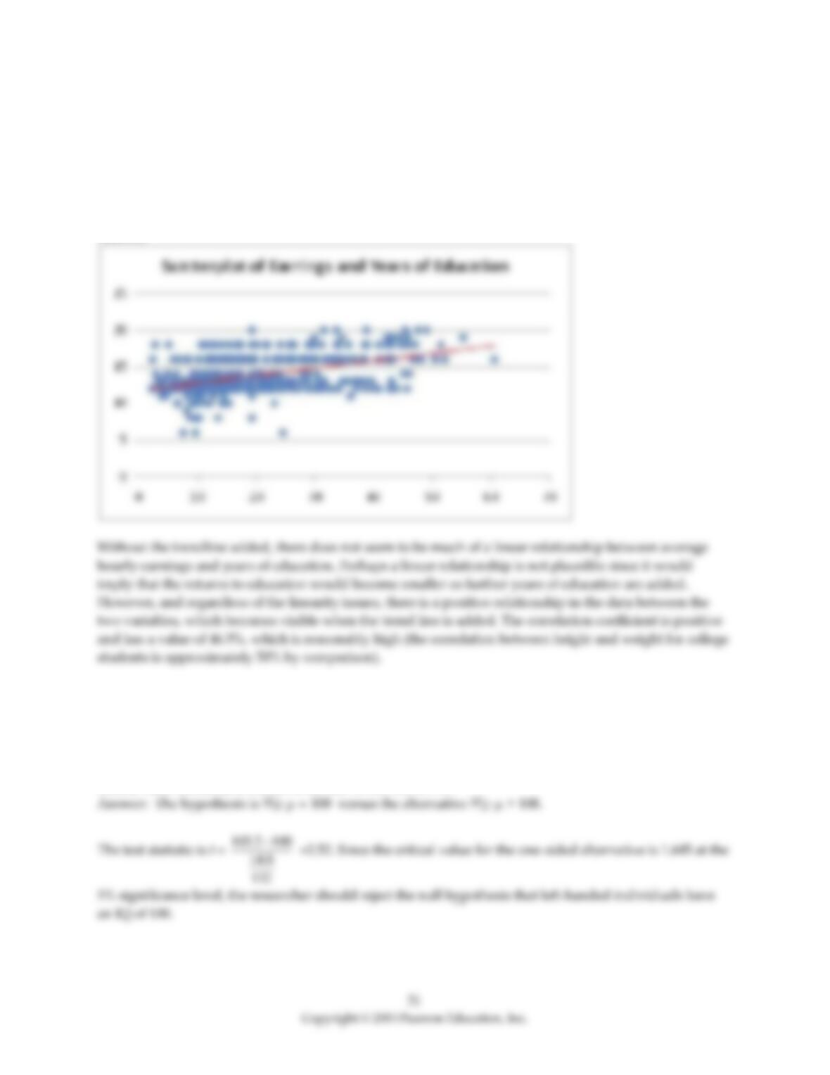
21) At the Stock and Watson (http://www.pearsonhighered.com/stock_watson) website go to Student
Resources and select the option “Datasets for Replicating Empirical Results.” Then select the chapter 8
CPS data set (ch8_cps.xls) into a spreadsheet program such as Excel. For the exercise, use the first 500
observations only. Using data for average hourly earnings only (ahe) and years of education (yrseduc),
produce a scatterplot with earnings on the vertical axis and education level on the horizontal axis. What
kind of relationship does the scatterplot suggest? Confirm your impression by adding a linear trendline.
Find the correlation coefficient between the two and interpret it.
Answer:
22) IQ scores are normally distributed with an average of 100 and a standard deviation of 16. Some
research suggests that left–handed individuals have a higher IQ score than right–handed individuals. To
test this hypothesis, a researcher randomly selects 132 individuals and finds that their average IQ is 103.2
with a sample standard deviation of 14.6. Using the results from the sample, can you reject the null
hypothesis that left–handed people have an IQ of 100 vs. the alternative that they have a higher IQ? What
critical value should you choose if the size of the test is 5%?
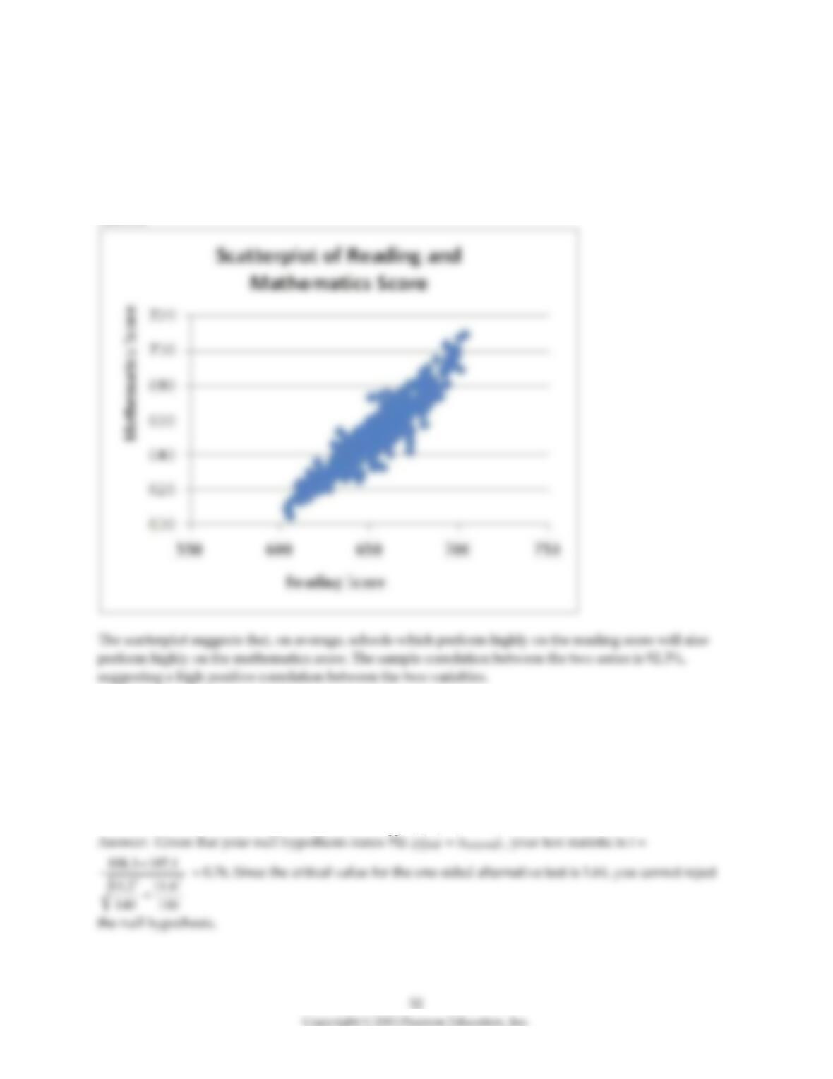
23) At the Stock and Watson (http://www.pearsonhighered.com/stock_watson) website go to Student
Resources and select the option “Datasets for Replicating Empirical Results.” Then select the “Test Score
data set used in Chapters 4–9″ (caschool.xls) and open the Excel data set. Next produce a scatterplot of the
average reading score (horizontal axis) and the average mathematics score (vertical axis). What does the
scatterplot suggest? Calculate the correlation coefficient between the two series and give an
interpretation.
Answer:
24) In 2007, a study of close to 250,000 18–19 year–old Norwegian males found that first–borns have an IQ
that is 2.3 points higher than those who are second–born. To see if you can find a similar evidence at your
university, you collect data from 250 students, of which 140 are first–borns. After subjecting each of these
individuals to an IQ test, you find that the first–borns score 108.3 with a standard deviation of 13.2, while
the second borns achieve 107.1 with a standard deviation of 11.6. You hypothesize that first–borns and
second–borns in a university population have identical IQs against the one–sided alternative hypothesis
that first borns have higher IQs. Using a size of the test of 5%, what is your conclusion?