Introduction to Econometrics, 3e (Stock)
Chapter 17 The Theory of Linear Regression with One Regressor
17.1 Multiple Choice
1) All of the following are good reasons for an applied econometrician to learn some econometric theory,
with the exception of
A) turning your statistical software from a “black box” into a flexible toolkit from which you are able to
select the right tool for a given job.
B) understanding econometric theory lets you appreciate why these tools work and what assumptions are
required for each tool to work properly.
C) learning how to invert a 4×4 matrix by hand.
D) helping you recognize when a tool will not work well in an application and when it is time for you to
look for a different econometric approach.
2) Finite–sample distributions of the OLS estimator and t–statistics are complicated, unless
A) the regressors are all normally distributed.
B) the regression errors are homoskedastic and normally distributed, conditional on X1,… Xn.
C) the Gauss–Markov Theorem applies.
D) the regressor is also endogenous.
3) If, in addition to the least squares assumptions made in the previous chapter on the simple regression
model, the errors are homoskedastic, then the OLS estimator is
A) identical to the TSLS estimator.
B) BLUE.
C) inconsistent.
D) different from the OLS estimator in the presence of heteroskedasticity.
4) When the errors are heteroskedastic, then
A) WLS is efficient in large samples, if the functional form of the heteroskedasticity is known.
B) OLS is biased.
C) OLS is still efficient as long as there is no serial correlation in the error terms.
D) weighted least squares is efficient.
5) The following is not part of the extended least squares assumptions for regression with a single
regressor:
A) var(ui Xi) = .
B) E(ui Xi) = 0.
C) the conditional distribution of ui given Xi is normal.
D) var(ui Xi) = .
6) The extended least squares assumptions are of interest, because
A) they will often hold in practice.
B) if they hold, then OLS is consistent.
C) they allow you to study additional theoretical properties of OLS.
D) if they hold, we can no longer calculate confidence intervals.
7) Asymptotic distribution theory is
A) not practically relevant, because we never have an infinite number of observations.
B) only of theoretical interest.
C) of interest because it tells you what the distribution approximately looks like in small samples.
D) the distribution of statistics when the sample size is very large.
8) Besides the Central Limit Theorem, the other cornerstone of asymptotic distribution theory is the
A) normal distribution.
B) OLS estimator.
C) Law of Large Numbers.
D) Slutsky’s theorem.
9) The link between the variance of and the probability that is within (± δ of is provided by
A) Slutsky’s theorem.
B) the Central Limit Theorem.
C) the Law of Large Numbers.
D) Chebychev’s inequality.
10) It is possible for an estimator of to be inconsistent while
A) converging in probability to .
B) Sn .
C) unbiased.
D) Pr → 0.
11) Slutsky’s theorem combines the Law of Large Numbers
A) with continuous functions.
B) and the normal distribution.
C) and the Central Limit Theorem.
D) with conditions for the unbiasedness of an estimator.
12) An implication of ( 1 – 1) N(0, ) is that
A) 1 is unbiased.
B) 1 is consistent.
C) OLS is BLUE.
D) there is heteroskedasticity in the errors.
13) Under the five extended least squares assumptions, the homoskedasticity–only t–distribution in this
chapter
A) has a Student t distribution with n–2 degrees of freedom.
B) has a normal distribution.
C) converges in distribution to a distribution.
D) has a Student t distribution with n degrees of freedom.
14) You need to adjust by the degrees of freedom to ensure that is
A) an unbiased estimator of .
B) a consistent estimator of .
C) efficient in small samples.
D) F–distributed.
15) E
A) is the expected value of the homoskedasticity only standard errors.
B) = .
C) exists only asymptotically.
D) = /(n–2).
16) The Gauss–Markov Theorem proves that
A) the OLS estimator is t distributed.
B) the OLS estimator has the smallest mean square error.
C) the OLS estimator is unbiased.
D) with homoskedastic errors, the OLS estimator has the smallest variance in the class of linear and
unbiased estimators, conditional on X1,…, Xn.
17) The following is not one of the Gauss–Markov conditions:
A) var(uiX1,…, Xn) = , 0 < < ∞ for i = 1,…, n,
B) the errors are normally distributed.
C) E(uiujX1,…, Xn) = 0, i = 1,…, n, j = 1,…, n, i ≠ j
D) E(uiX1,…, Xn) = 0
18) The class of linear conditionally unbiased estimators consists of
A) all estimators of β1 that are linear functions of Y1,…, Yn and that are unbiased, conditional on X1,…,
Xn .
B) OLS, WLS, and TSLS.
C) those estimators that are asymptotically normally distributed.
D) all estimators of β1 that are linear functions of X1,…, Xn and that are unbiased, conditional on X1,…,
Xn.
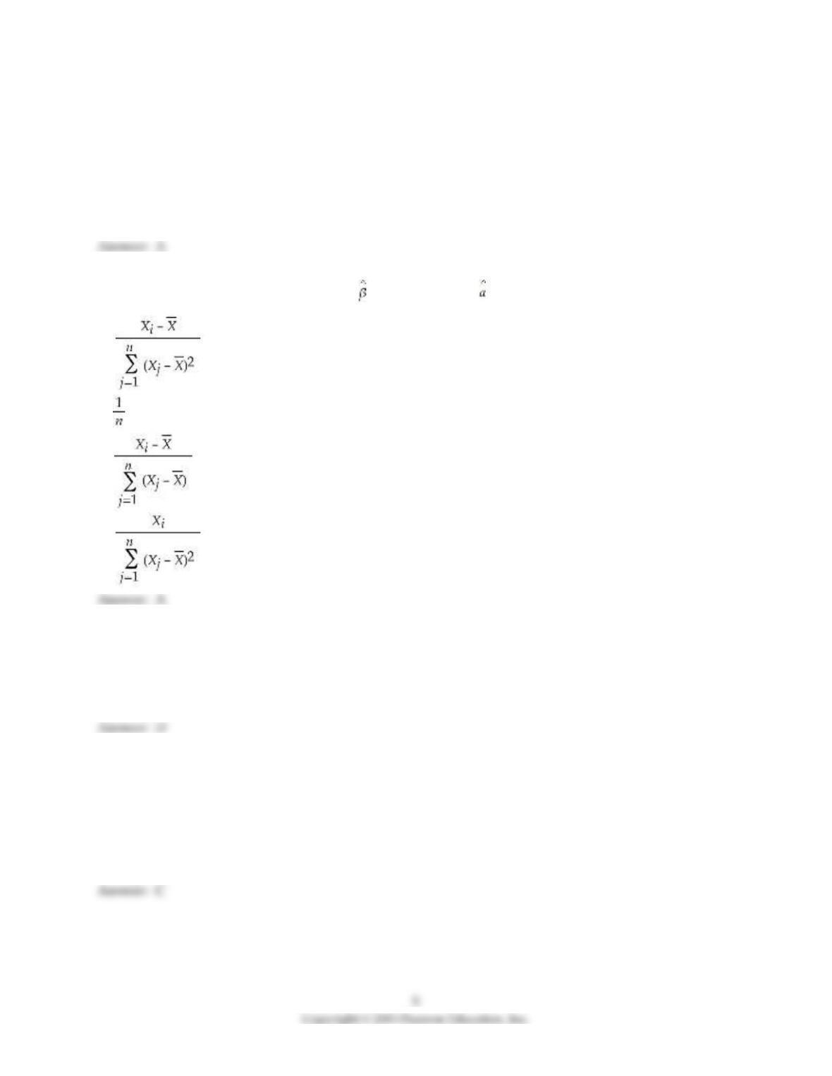
19) The OLS estimator is a linear estimator, 1 =
1
ˆ
n
ii
i
aY
=
, where i =
A) .
B) .
C) .
D) .
20) If the errors are heteroskedastic, then
A) the OLS estimator is still BLUE as long as the regressors are nonrandom.
B) the usual formula cannot be used for the OLS estimator.
C) your model becomes overidentified.
D) the OLS estimator is not BLUE.
21) Estimation by WLS
A) although harder than OLS, will always produce a smaller variance.
B) does not mean that you should use homoskedasticity–only standard errors on the transformed
equation.
C) requires quite a bit of knowledge about the conditional variance function.
D) makes it very hard to interpret the coefficients, since the data is now weighted and not any longer in
its original form.
22) The WLS estimator is called infeasible WLS estimator when
A) the memory required to compute it on your PC is insufficient.
B) the conditional variance function is not known.
C) the numbers used to compute the estimator get too large.
D) calculating the weights requires you to take a square root of a negative number.
23) Feasible WLS does not rely on the following condition:
A) the conditional variance depends on a variable which does not have to appear in the regression
function.
B) estimating the conditional variance function.
C) the key assumptions for OLS estimation have to apply when estimating the conditional variance
function.
D) the conditional variance depends on a variable which appears in the regression function.
24) In practice, the most difficult aspect of feasible WLS estimation is
A) knowing the functional form of the conditional variance.
B) applying the WLS rather than the OLS formula.
C) finding an econometric package that actually calculates WLS.
D) applying WLS when you have a log–log functional form.
25) The advantage of using heteroskedasticity–robust standard errors is that
A) they are easier to compute than the homoskedasticity–only standard errors.
B) they produce asymptotically valid inferences even if you do not know the form of the conditional
variance function.
C) it makes the OLS estimator BLUE, even in the presence of heteroskedasticity.
D) they do not unnecessarily complicate matters, since in real–world applications, the functional form of
the conditional variance can easily be found.
26) Homoskedasticity means that
A) var(ui|Xi) =
B) var(Xi) =
C) var(ui|Xi) =
D) var( i|Xi) =
27) In order to use the t–statistic for hypothesis testing and constructing a 95% confidence interval as
1.96 standard errors, the following three assumptions have to hold:
A) the conditional mean of ui, given Xi is zero; (Xi,Yi), i = 1,2, …, n are i.i.d. draws from their joint
distribution; Xi and ui have four moments
B) the conditional mean of ui, given Xi is zero; (Xi,Yi), i = 1,2, …, n are i.i.d. draws from their joint
distribution; homoskedasticity
C) the conditional mean of ui, given Xi is zero; (Xi,Yi), i = 1,2, …, n are i.i.d. draws from their joint
distribution; the conditional distribution of ui given Xi is normal
D) none of the above
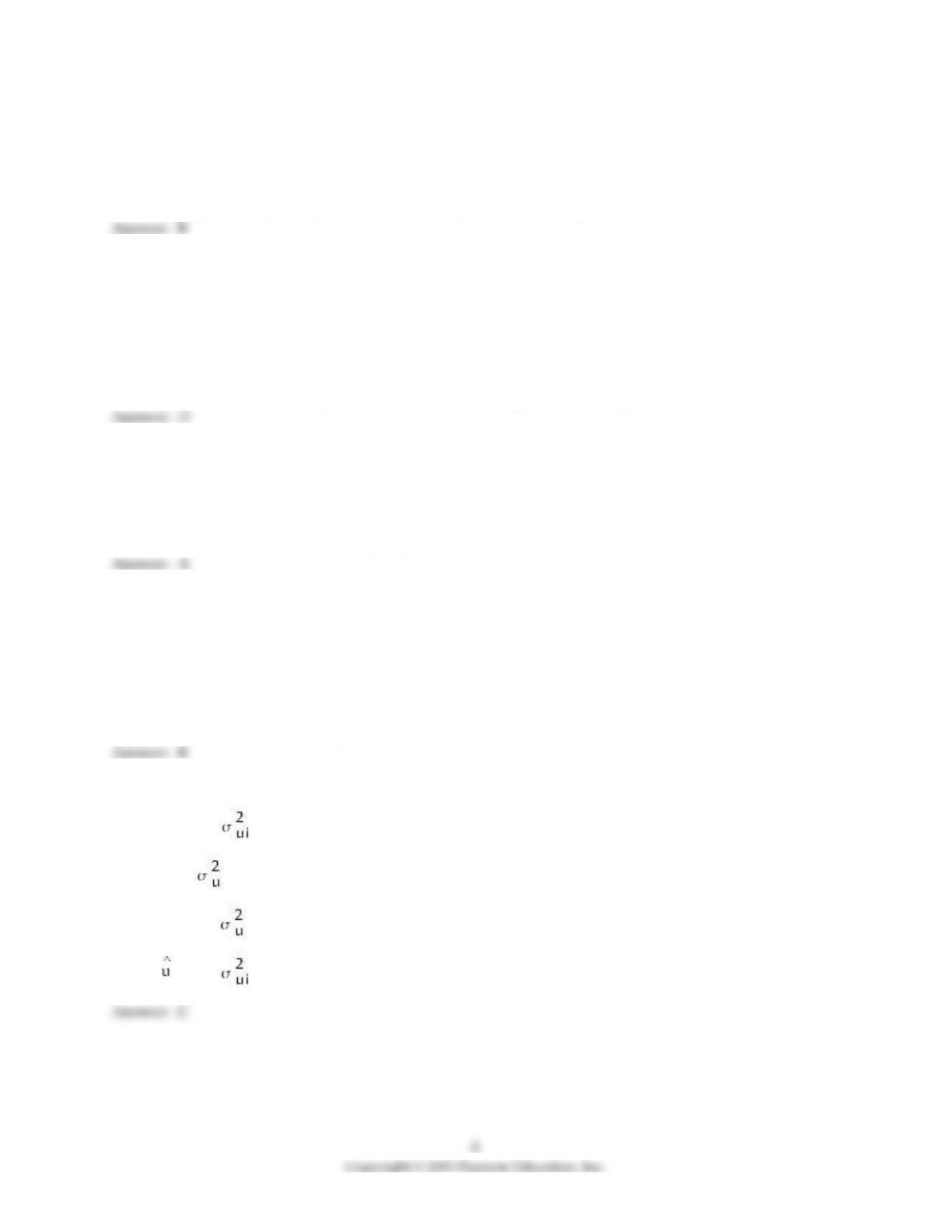
28) If the variance of u is quadratic in X, then it can be expressed as
A) var(ui|Xi) =
B) var(ui|Xi) = θ0 + θ1
C) var(ui|Xi) = θ0 + θ1
D) var(ui|Xi) =
29) In practice, you may want to use the OLS estimator instead of the WLS because
A) heteroskedasticity is seldom a realistic problem
B) OLS is easier to calculate
C) heteroskedasticity robust standard errors can be calculated
D) the functional form of the conditional variance function is rarely known
30) If the functional form of the conditional variance function is incorrect, then
A) the standard errors computed by WLS regression routines are invalid
B) the OLS estimator is biased
C) instrumental variable techniques have to be used
D) the regression R2 can no longer be computed
8
Copyright © 2015 Pearson Education, Inc.
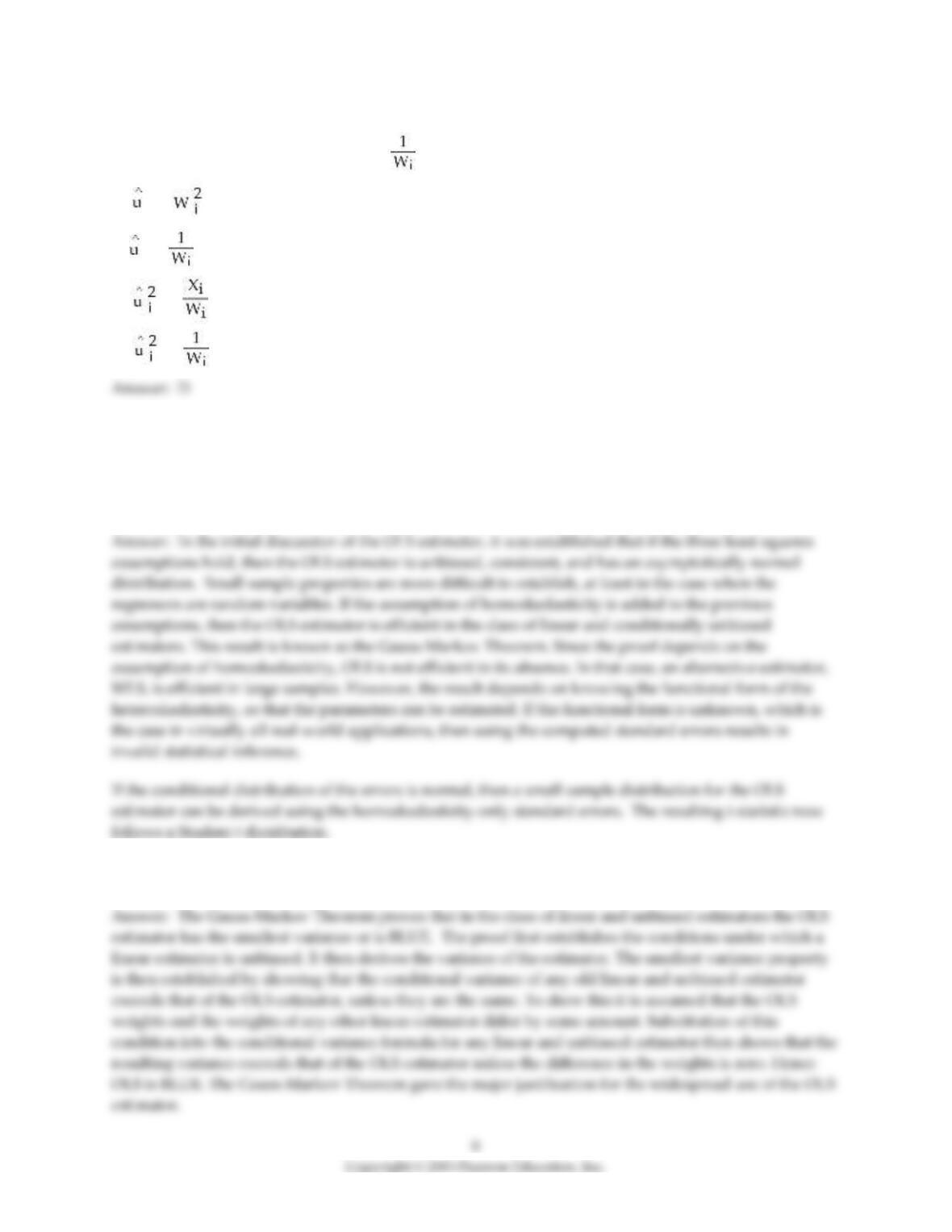
31) Suppose that the conditional variance is var(ui|Xi) = λh(Xi) where λ is a constant and h is a known
function. The WLS estimator is
A) the same as the OLS estimator since the function is known
B) can only be calculated if you have at least 100 observations
C) the estimator obtained by first dividing the dependent variable and regressor by the square root of h
and then regressing this modified dependent variable on the modified regressor using OLS
D) the estimator obtained by first dividing the dependent variable and regressor by h and then regressing
this modified dependent variable on the modified regressor using OLS
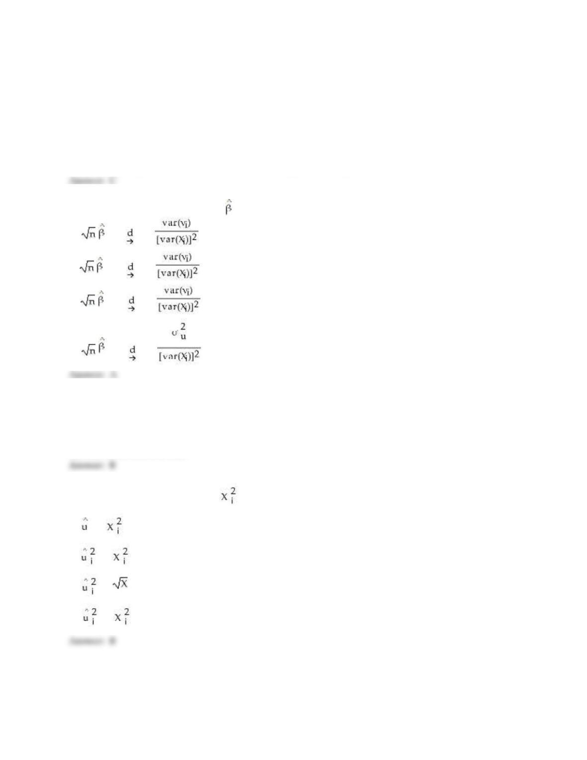
32) The large–sample distribution of 1 is
A) ( 1–β1) N(0 where νi= (Xi–μx)ui
B) ( 1–β1) N(0 where νi= ui
C) ( 1–β1) N(0 where νi= Xiui
D) ( 1–β1) N(0
33) (Requires Appendix material) If X and Y are jointly normally distributed and are uncorrelated,
A) then their product is chi–square distributed with n–2 degrees of freedom
B) then they are independently distributed
C) then their ratio is t–distributed
D) none of the above is true
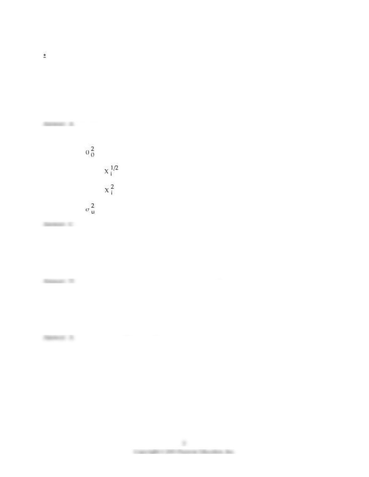
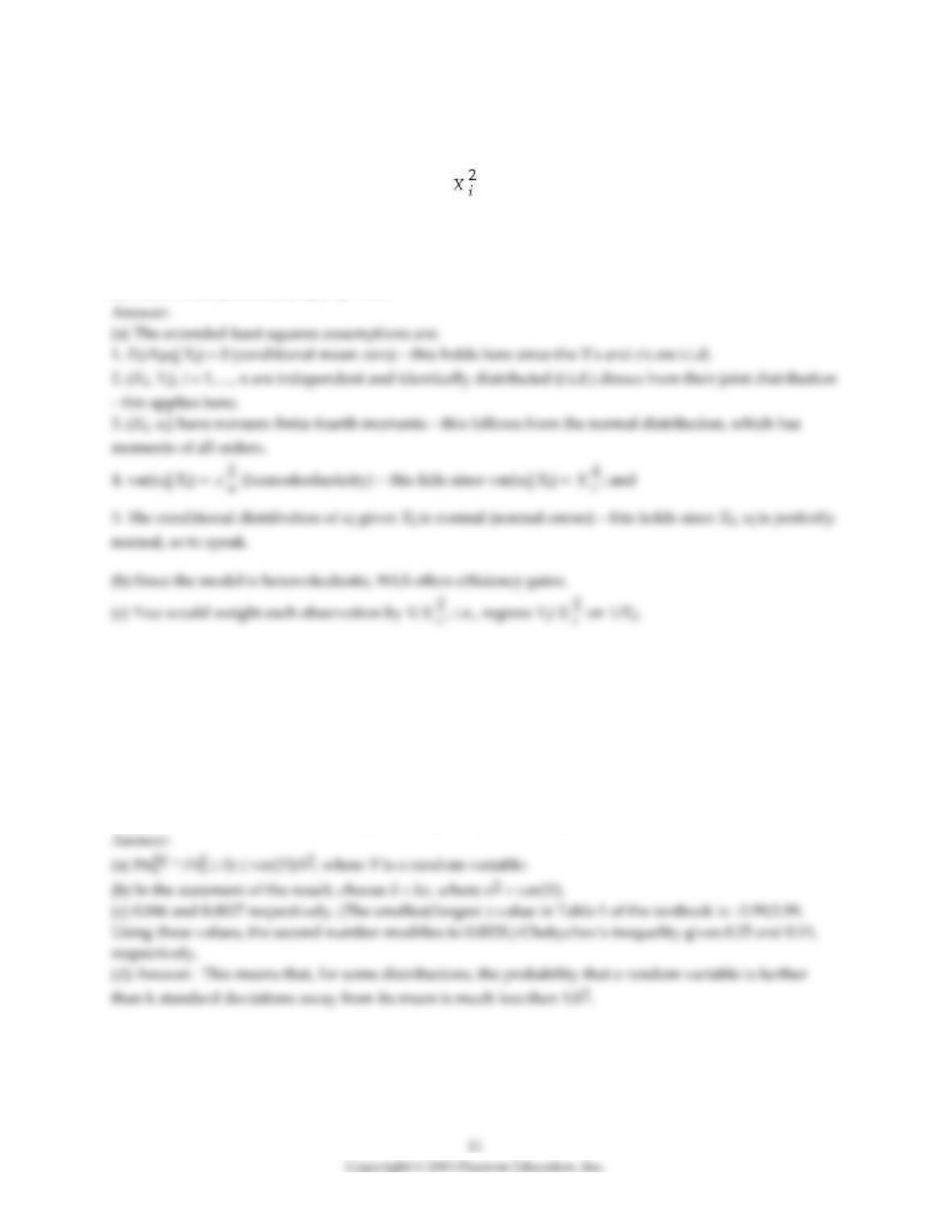
34) Assume that var(ui|Xi) = θ0+θ1. One way to estimate θ0 and θ1 consistently is to regress
A) i on using OLS
B) on using OLS
C) on iusing OLS
D) on using OLS but suppressing the constant (“restricted least squares”)
35) Assume that the variance depends on a third variable, Wi, which does not appear in the regression
function, and that var(ui|Xi,Wi) = θ0+θ1. One way to estimate θ0 and θ1consistently is to regress
A) i on using OLS
B) i on
using OLS
C) on using OLS
D) on using OLS
17.2 Essays and Longer Questions
1) Discuss the properties of the OLS estimator when the regression errors are homoskedastic and
normally distributed. What can you say about the distribution of the OLS estimator when these features
are absent?
2) What does the Gauss–Markov theorem prove? Without giving mathematical details, explain how the
proof proceeds. What is its importance?
3) One of the earlier textbooks in econometrics, first published in 1971, compared “estimation of a
parameter to shooting at a target with a rifle. The bull’s–eye can be taken to represent the true value of the
parameter, the rifle the estimator, and each shot a particular estimate.” Use this analogy to discuss small
and large sample properties of estimators. How do you think the author approached the n → ∞
condition? (Dependent on your view of the world, feel free to substitute guns with bow and arrow, or
missile.)
4) “I am an applied econometrician and therefore should not have to deal with econometric theory. There
will be others who I leave that to. I am more interested in interpreting the estimation results.” Evaluate.
5) “One should never bother with WLS. Using OLS with robust standard errors gives correct inference, at
least asymptotically.” True, false, or a bit of both? Explain carefully what the quote means and evaluate it
critically.
17.3 Mathematical and Graphical Problems
1) Consider the model Yi = β1Xi + ui, where ui = c ei and all of the X‘s and e‘s are i.i.d. and distributed
N(0,1).
(a) Which of the Extended Least Squares Assumptions are satisfied here? Prove your assertions.
(b) Would an OLS estimator of β1 be efficient here?
(c) How would you estimate β1 by WLS?
2) (Requires Appendix material) This question requires you to work with Chebychev‘s Inequality.
(a) State Chebychev’s Inequality.
(b) Chebychev’s Inequality is sometimes stated in the form “The probability that a random variable is
further than k standard deviations from its mean is less than 1/k2.” Deduce this form. (Hint: choose δ
artfully.)
(c) If X is distributed N(0,1), what is the probability that X is two standard deviations from its mean?
Three? What is the Chebychev bound for these values?
(d) It is sometimes said that the Chebychev inequality is not “sharp.” What does that mean?
12
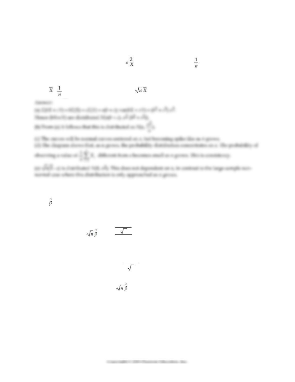
3) For this question you may assume that linear combinations of normal variates are themselves normally
distributed. Let a, b, and c be non–zero constants.
(a) X and Y are independently distributed as N(a, σ2). What is the distribution of (bX+cY)?
(b) If X1,…, Xn are distributed i.i.d. as N(a, ), what is the distribution of
1
n
i
i
X
=
?
(c) Draw this distribution for different values of n. What is the asymptotic distribution of this statistic?
(d) Comment on the relationship between your diagram and the concept of consistency.
(e) Let =
1
n
i
i
X
=
1
n
i
i
X
=
. What is the distribution of ( – a)? Does your answer depend on n?
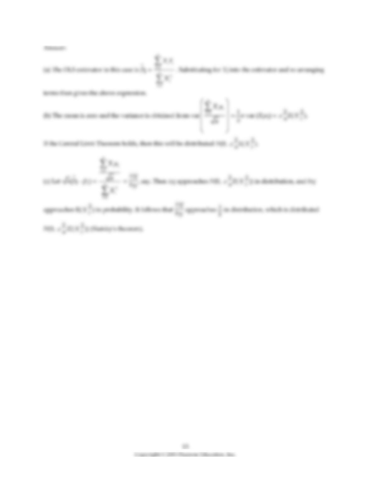
4) Consider the model Yi – β1Xi + ui, where the Xi and ui the are mutually independent i.i.d. random
variables with finite fourth moment and E(ui) = 0.
(a) Let 1 denote the OLS estimator of β1. Show that
( 1– β1) =
1
2
1
n
ii
i
n
i
i
Xu
n
X
=
=
.
(b) What is the mean and the variance of
1
n
ii
i
Xu
n
=
? Assuming that the Central Limit Theorem holds, what
is its limiting distribution?
(c) Deduce the limiting distribution of ( 1 – β1)? State what theorems are necessary for your deduction.
1
n
i
i
a
=
1
n
ii
i
aX
=
1
n
i
i
a
=
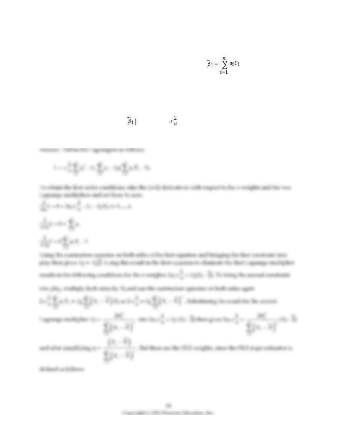
5) (Requires Appendix material) If the Gauss–Markov conditions hold, then OLS is BLUE. In addition,
assume here that X is nonrandom. Your textbook proves the Gauss–Markov theorem by using the simple
regression model Yi = β0 + β1Xi + ui and assuming a linear estimator . Substitution of the
simple regression model into this expression then results in two conditions for the unbiasedness of the
estimator:
1
n
i
i
a
=
= 0 and
1
n
ii
i
aX
=
= 1.
The variance of the estimator is var( X1,…, Xn) =
2
1
n
i
i
a
=
.
Different from your textbook, use the Lagrangian method to minimize the variance subject to the two
constraints. Show that the resulting weights correspond to the OLS weights.
nn
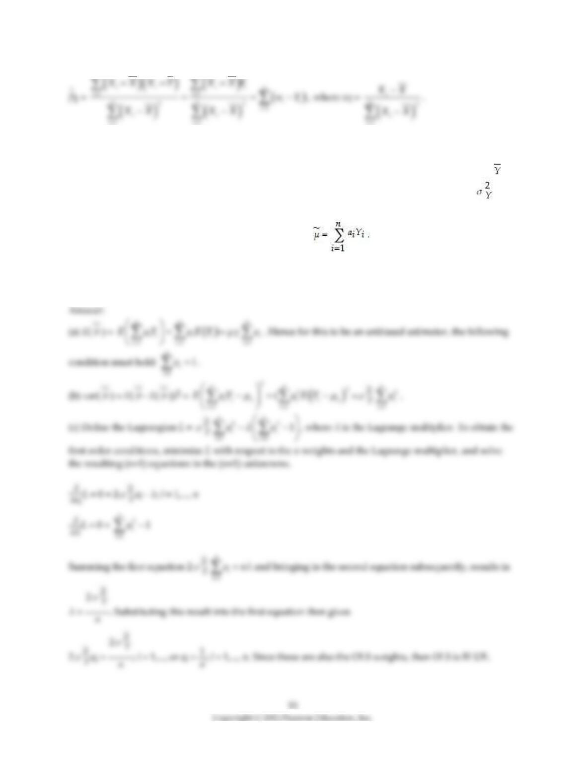
6) Your textbook states that an implication of the Gauss–Markov theorem is that the sample average, , is
the most efficient linear estimator of E(Yi) when Y1,…, Yn are i.i.d. with E(Yi) = μY and var(Yi) = .
This follows from the regression model with no slope and the fact that the OLS estimator is BLUE.
Provide a proof by assuming a linear estimator in the Y‘s,
(a) State the condition under which this estimator is unbiased.
(b) Derive the variance of this estimator.
(c) Minimize this variance subject to the constraint (condition) derived in (a) and show that the sample
mean is BLUE.
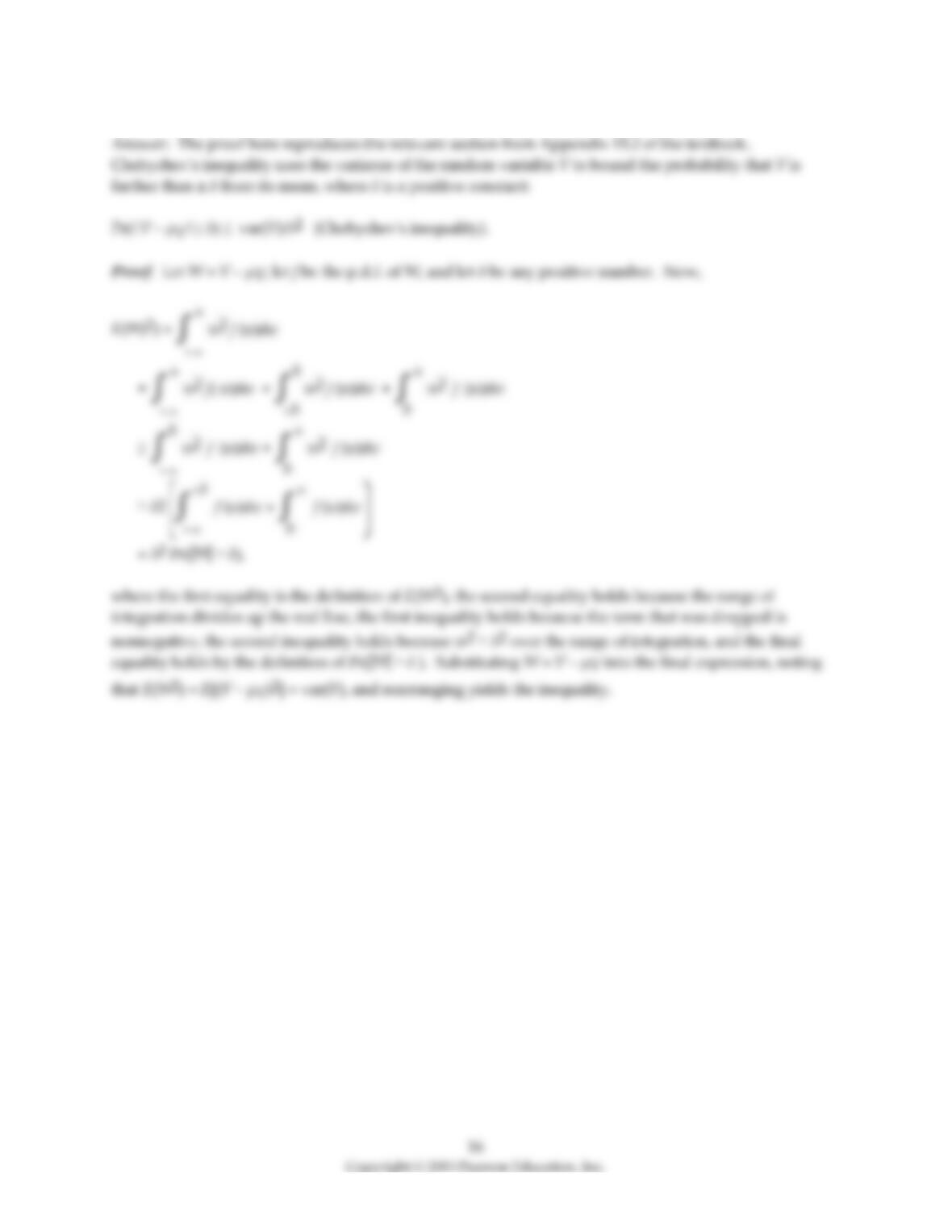
7) (Requires Appendix material) State and prove the Cauchy–Schwarz Inequality.
17
8) Consider the simple regression model Yi = β0 + β1Xi + ui where Xi > 0 for all i, and the conditional
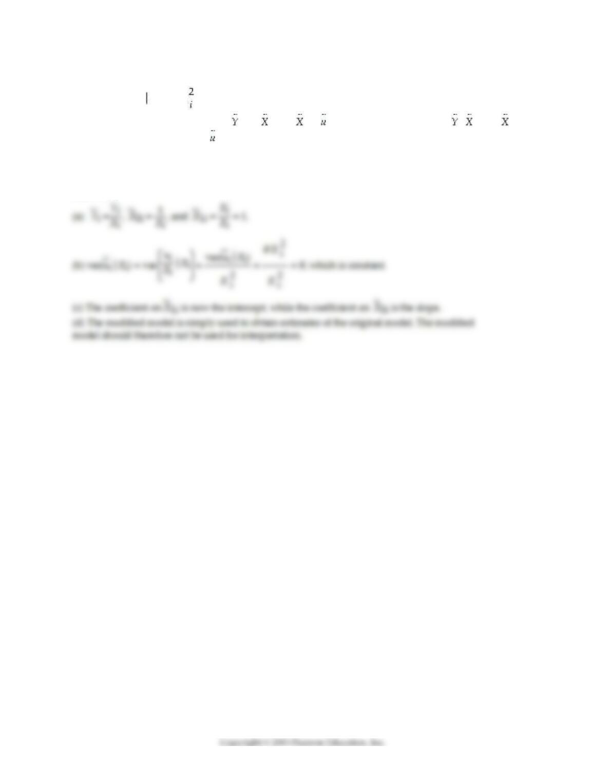
variance is var(uiXi) = θX where θ is a known constant with θ > 0.
(a) Write the weighted regression as i = β0 0i + β1 1i + i. How would you construct i, 0i and 1i?
(b) Prove that the variance of is i homoskedastic.
(c) Which coefficient is the intercept in the modified regression model? Which is the slope?
(d) When interpreting the regression results, which of the two equations should you use, the original or
the modified model?
Answer:
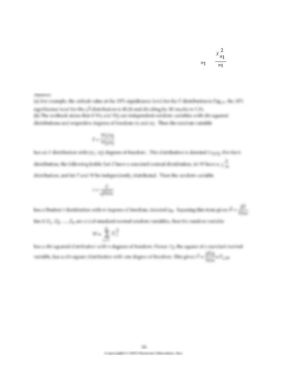
9) (Requires Appendix material) Your textbook considers various distributions such as the standard
normal, t, χ2, and F distribution, and relationships between them.
(a) Using statistical tables, give examples that the following relationship holds: F,∞ = .
(b) t∞ is distributed standard normal, and the square of the t–distribution with n2 degrees of freedom
equals the value of the F distribution with (1, n2) degrees of freedom. Why does this relationship between
the t and F distribution hold?
10) Consider estimating a consumption function from a large cross–section sample of households.
Assume that households at lower income levels do not have as much discretion for consumption
variation as households with high income levels. After all, if you live below the poverty line, then almost
all of your income is spent on necessities, and there is little room to save. On the other hand, if your
annual income was $1 million, you could save quite a bit if you were a frugal person, or spend it all, if
you prefer. Sketch what the scatterplot between consumption and income would look like in such a
situation. What functional form do you think could approximate the conditional variance var(ui Inome)?