16
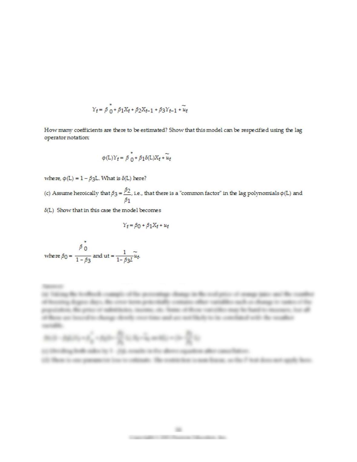
5) Your textbook used a distributed lag model with only current and past values of Xt–1 coupled with an
AR(1) error model to derive a quasi–difference model, where the error term was uncorrelated.
(a) Instead use a static model Yt = β0 + β1Xt + ut here, where the error term follows an AR(1). Derive the
quasi difference form. Explain why in the case of the infeasible GLS estimators you could easily estimate
the βs by OLS.
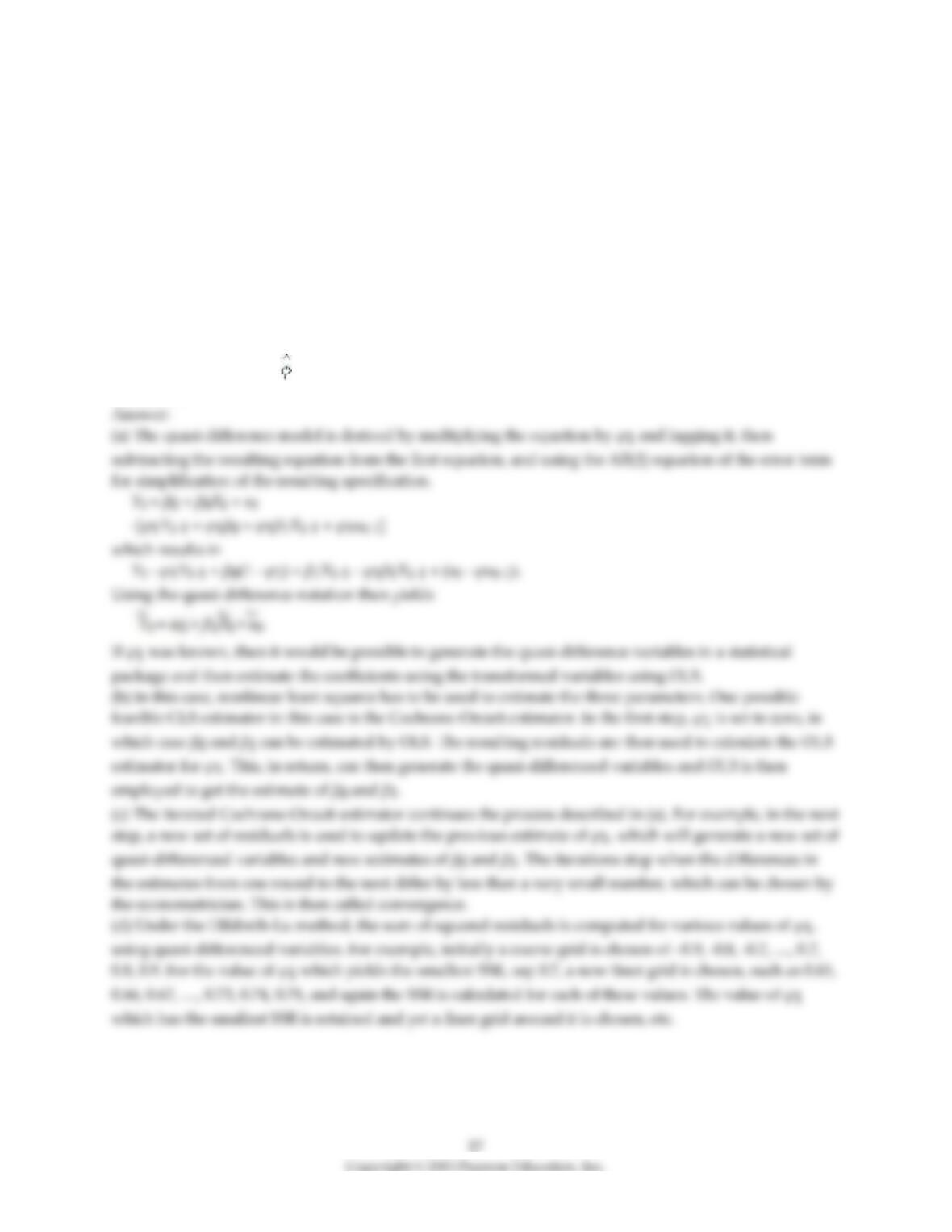
(b) Since φ1 (the autocorrelation parameter for ut) is unknown, describe the Cochrane–Orcutt estimation
procedure.
(c) Explain how the iterated Cochrane–Orcutt estimator works in this situation. Iterations stop when there
is “convergence” in the estimates. What do you think is meant by that?
(d) Your textbook has pointed out that the iterated Cochrane–Orcutt GLS estimator is in fact the nonlinear
least squares estimator of the model. Given that –1 < φ1 < 1, suggest a “grid search” or some strategy to
“nail down” the value of 1 which minimizes the sum of squared residuals. This is the so–called Hildreth–
Lu method.
6) (Requires Appendix material) Your textbook states that in “the distributed lag regression model, the
error term ut can be correlated with its lagged values. This autocorrelation arises, because, in time series
data, the omitted factors that comprise ut can themselves be serially correlated.”
(a) Give an example what the authors have in mind.
(b) Consider the ADL model, where the X‘s are strictly exogenous, and there is no autocorrelation (and/or
heteroskedasticity) in the error term.
(d) Explain why autocorrelation in this model can be seen as a “simplification,” not a “nuisance.” Can you
use the F–test to test the above hypothesis? Why or why not?

7) It has been argued that Canada‘s aggregate output growth and unemployment rates are very sensitive
to United States economic fluctuations, while the opposite is not true.
(a) A researcher uses a distributed lag model to estimate dynamic causal effects of U.S. economic activity
on Canada. The results (HAC standard errors in parenthesis) for the sample period 1961:I–1995:IV are:
t = –1.42 + 0.717 × urust + 0.262 × urust–1 + 0.023 × urust–2 – 0.083 × urust–3
(0.83) (0.457) (0.557) (0.398) (0.405)
– 0.726 × urust–4 + 1.267 × urust–5; R2= 0.672, SER = 1.444
(0.504) (0.385)
where urcan is the Canadian unemployment rate, and urus is the United States unemployment rate.
Calculate the long–run cumulative dynamic multiplier.
(b) What are some of the omitted variables that could cause autocorrelation in the error terms? Are these
omitted variables likely to uncorrelated with current and lagged values of the U.S. unemployment rate?
Do you think that the U.S. unemployment rate is exogenous in this distributed lag regression?
22
9) The distributed lag regression model requires estimation of (r+1) coefficients in the case of a single
explanatory variable. In your textbook example of orange juice prices and cold weather, r = 18. With
additional explanatory variables, this number becomes even larger.
Consider the distributed lag regression model with a single regressor
Yt = β0 + β1Xt + β2Xt–1 + β3Xt–2 + … + βr+1Xt–r + ut
(a) Early econometric analysis of distributed lag regression models was interested in reducing the
number of parameters by approximating the coefficients by a polynomial of a suitable degree, i.e., βi+1 ≈
f(i) for i = 0, 1, …, r. Let f(i) be a third degree polynomial, with coefficients α0, …., α3. Specify the
equations for β1, β2, β3, β4, and βr+1.
(b) Substitute these equations into the original distributed lag regression, and rearrange terms so that Y
appears as a linear function of β0, α0, α1, α2, α3 and a transformation of the Xt, Xt–1, Xt–2, …, Xt–r
(c) Assume that the third–degree polynomial approximation is quite accurate. Then what is the advantage
of this polynomial lag technique?
Answer:
10) The distributed lag model relating orange juice prices to the Orlando weather reported in the text was
of the form
%ChgPt = β0 + β1FDDt + β2FDDt–1 + β3FDDt–2 + … + β19FDDt–18 + ut
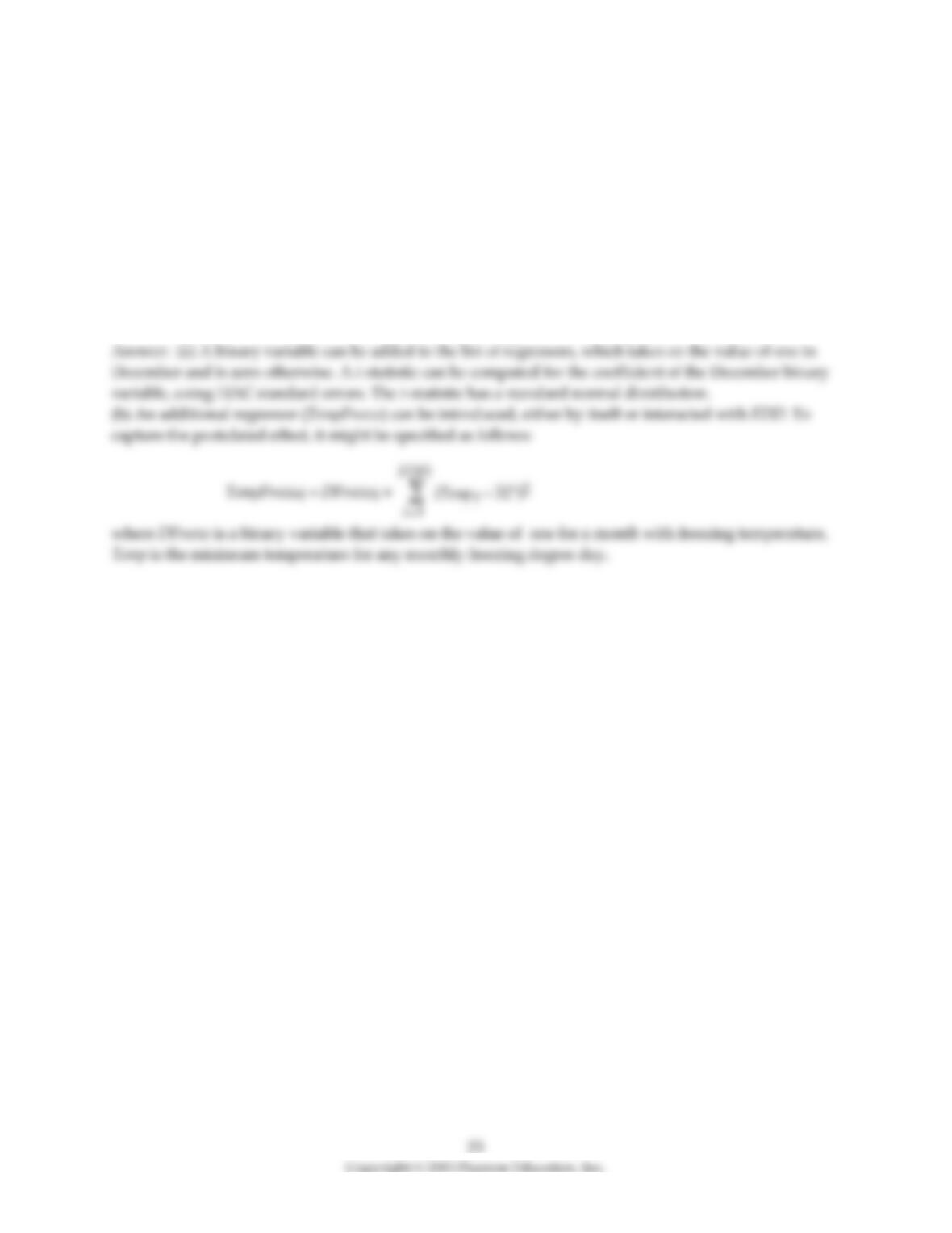
(a) Suppose that an agricultural economist tells you that a freeze in December is more harmful than a
freeze in the other months. How would you modify the regression to incorporate this effect? How
would you test for this December effect?
(b) The same economist tells you that the damage caused by freezes is not well captured by the FDD
variable. She says that a single day temperature with a temperature of 24° is more damaging than 8 days
with a temperature of 31°. How would you modify the regression to incorporate this effect?
11) (Requires some calculus) In the following, assume that Xt is strictly exogenous and that economic
theory suggests that, in equilibrium, the following relationship holds between Y* and Xt, where the “*”
indicates equilibrium.
Y* = kXt
An error term could be added here by assuming that even in equilibrium, random variations from strict
proportionality might occur. Next let there be adjustment costs when changing Y, e.g. costs associated
with changes in employment for firms. As a result, an entity might be faced with two types of costs: being
out of equilibrium and the adjustment cost. Assume that these costs can be modeled by the following
quadratic loss function:
L = λ1(Yt — Y*)2 + λ1(Yt — Yt–1)2
a. Minimize the loss function w.r.t. the only variable that is under the entity’s control, Yt and solve for Yt.
b. Note that the two weights on Y* and Yt–1 add up to one. To simplify notation, let the first weight be θ
and the second weight (1–θ). Substitute the original expression for Y* into this equation. In terms of the
ADL(p,q) terminology, what are the values for p and q in this model?
12) Your textbook estimates the initial relationship between the percentage change of real frozen OJ and
the freezing degree days as follows:
t = –0.40 + 0.47 FDDt
(0.22) (0.13)
t = 1950:1 — 2000:12, R2 = 0.09, SER = 4.8
a. Calculate the t–statistic for the slope coefficient. Can you reject the null hypothesis that the coefficient is
zero in the population?
b. The above regression was estimated using HAC standard errors. When you re–estimate the regression
using homoskedasticity–only standard errors, the standard error of the slope coefficient drops to 0.06.
Calculate the t–statistic for the slope coefficient again. Which of the two standard errors should you use
for statistical inference?
13) You are hired to forecast the unemployment rate in a geographical area that is peripheral to a large
metropolitan area in the United States. The area in question is called the Inland Empire (San Bernardino
County and Riverside County) and is situated east of Greater Los Angeles (Los Angeles County and
Orange County). While the area has a large population (it is the 14th largest metropolitan statistical area in
the United States), its economic activity relies heavily on that of the larger area it is attached to. For
example, it is estimated that approximately 20% of its workforce commutes into the Greater Los Angeles
area for work and few workers commute the other way. Furthermore, its logistics industry is heavily
dependent on economic activity in the Greater Los Angeles Area. As a result, you view the
unemployment rate of the Greater Los Angeles Area (urGLA) to be exogenous in determining the
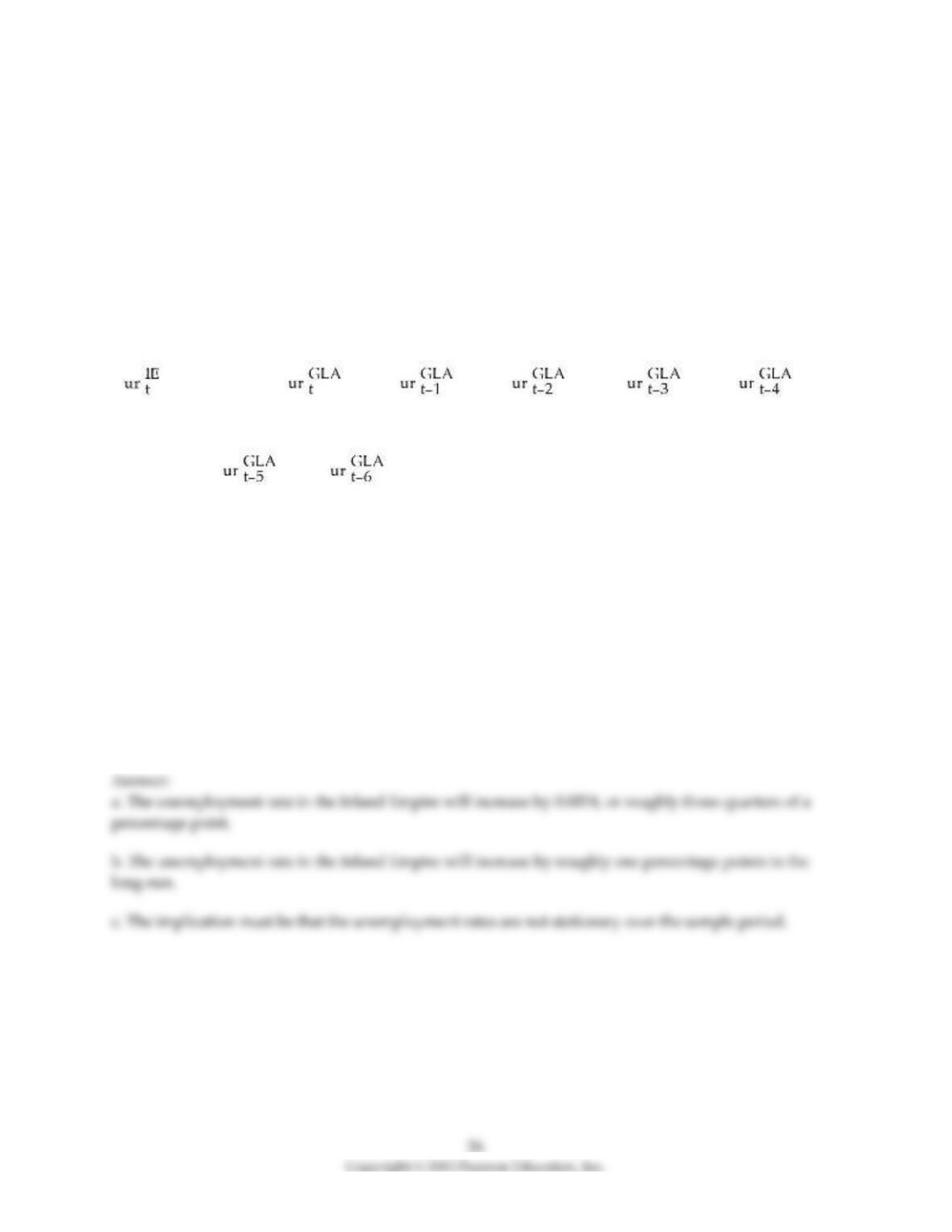
unemployment rate in the Inland Empire (urIE). You estimate the following distributed lag model, where
numbers in parenthesis are HAC standard errors:
Δ = 0.00002 + 0.74 Δ – 0.04 Δ – 0.01 Δ + 0.07 Δ + 0.05 Δ
(0.00010) (0.06) (0.06) (0.06) (0.06) (0.06)
+ 0.09 Δ + 0.10Δ
(0.05) (0.06)
t = 1991:01–2009:12, R2 = 0.60, SER = 0.001
a. What is the impact effect of a one percentage point increase (say from 0.06 to 0.07) of the
unemployment rate in the Greater Los Angeles area?
b. What is the long–run cumulative dynamic multiplier?
c. Why do you think the variables above appear in changes rather than in levels?
14) There is some economic research which suggests that oil prices play a central role in causing
recessions in developed countries. Some of this work suggests that it is only oil price increases that matter
and even more specifically, that it is the percentage point difference between oil prices at date t and the
maximum value over the previous year. Realizing that energy prices in general can fluctuate quite
dramatically in both directions and that geographic areas also benefit substantially from oil price
decreases, you decide to estimate the following distributed lag model using annual data (numbers in
parenthesis are HAC standard errors):
t = 3.39 – 0.009 (Poil/CPI)t – 0.028 (Poil/CPI)t–1
(0.27) (0.010) (0.011)
t = 1960–2008, R2 = 0.15, SER = 1.88
a. What is the impact effect of a 25 percent increase in real oil prices?
b. What is the predicted cumulative change in GDP Growth over two years of this effect?
c. The HAC F–statistic is 4.07. Can you reject the null hypothesis that oil price changes have no effect on
real GDP growth? What is the critical value you considered? Is there any reason why you should be
cautious using an F–test in this case, given the sample period?