Unlock document.
This document is partially blurred.
Unlock all pages and 1 million more documents.
Get Access

13.3 Mathematical and Graphical Problems
1) Your textbook mentions use of a quasi-experiment to study the effects of minimum wages on
employment using data from fast food restaurants. In 1992, there was an increase in the (state) minimum
wage in one U.S. state (New Jersey) but not in neighboring location (Eastern Pennsylvania). To calculate
the you need the change in the treatment group and the change in the control group. To
do this, the study provides you with the following information
PA
NJ
FTE Employment
before
23.33
20.44
FTE Employment after
21.17
21.03
Where FTE is "full time equivalent" and the numbers are average employment per restaurant.
(a) Calculate the change in the treatment group, the change in the control group, and finally
. Since minimum wages represent a price floor, did you expect to be
positive or negative?
(b) If you look at , is this number primarily due to a change in the treatment group or the
control group? Is this what you expected?
(c) The standard error for is 1.36. Test whether or not the coefficient is statistically
significant, given that there are 410 observations. If you believed that the benefit from small minimum
wage increases outweighed the cost in terms of employment loss, would finding that this coefficient was
not statistically significant discourage you?

14
2) Define the in terms of observable differences in the treatment and control group, before
and after the treatment. Explain why this presentation is the equivalent of calculating the coefficient in a
regression framework.
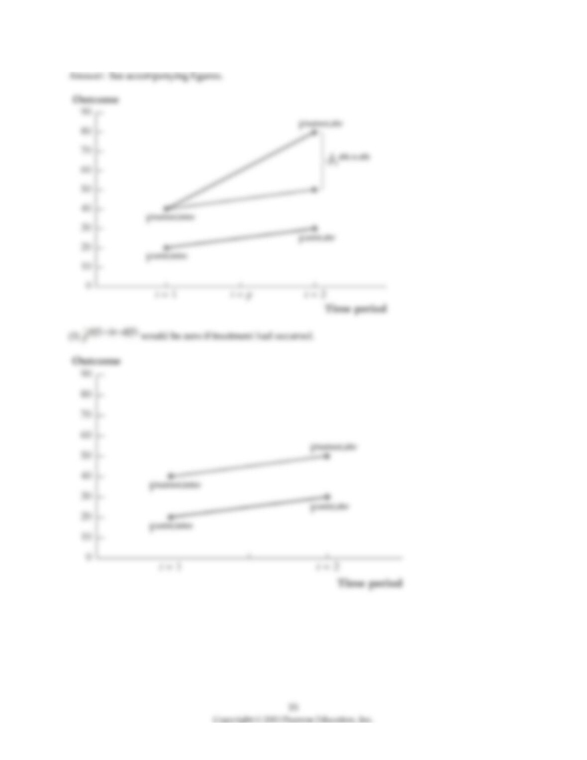
3) Your textbook gives a graphical example of , where outcome is plotted on the vertical
axis, and time period appears on the horizontal axis. There are two time periods entered: "t = 1"
and "t = 2." The former corresponds to the "before" time period, while the latter represents the "after"
period. The assumption is that the policy occurred sometime between the time periods (call this "t = p").
Keeping in mind the graphical example of , carefully read what a reviewer of the Card and
Krueger (CK) study of the minimum wage effect on employment in the New Jersey-Pennsylvania study
had to say:
"Two assumptions are implicit throughout the evaluation of the ‘natural experiment:' (1) [ ]
would be zero if the treatment had not occurred, so a nonzero [ ] indicates the effect of the
treatment (that is, nothing else could have caused the difference in the outcomes to change), and (2) …
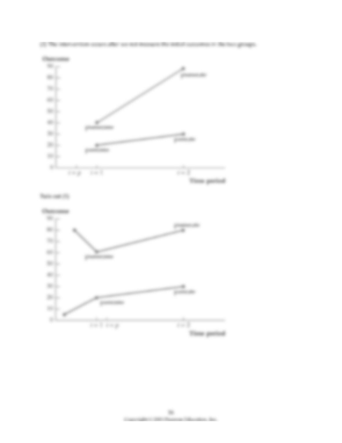
the intervention occurs after we measure the initial outcomes in the two groups. … Three conditions are
particularly relevant in interpreting CK's work: (1) [t = 1] must be sufficiently before [t = p] that [the
treatment group] did not adjust to the treatment before [t=1] – otherwise [ –
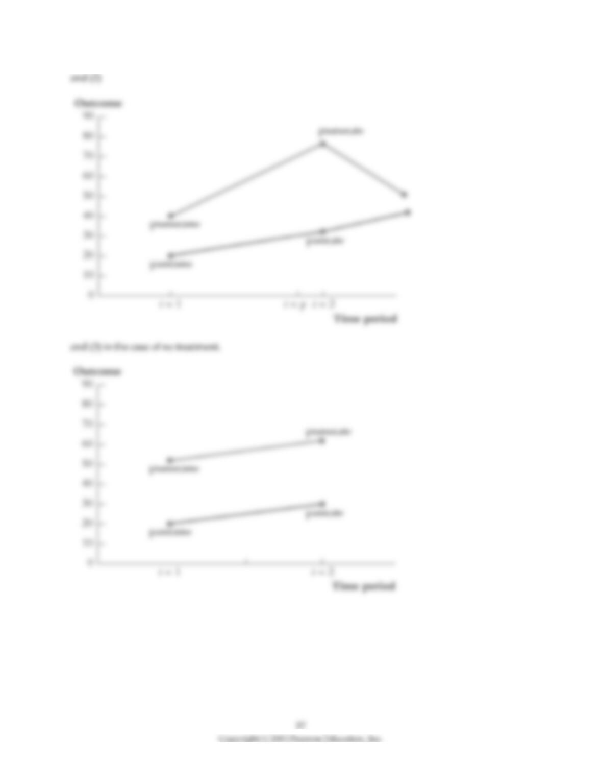
] will reflect the effect of the treatment; (2) [t = 2] must be sufficiently after [t = p] to allow
the treatment's effect to be fully felt; and (3) we must be sure that the same difference [ –
] would have been observed at [t = 2] if the treatment had not been imposed, that is, [the
control group must be good enough] that there is no need to adjust the differences for factors other than
the treatment that might have caused them to change."
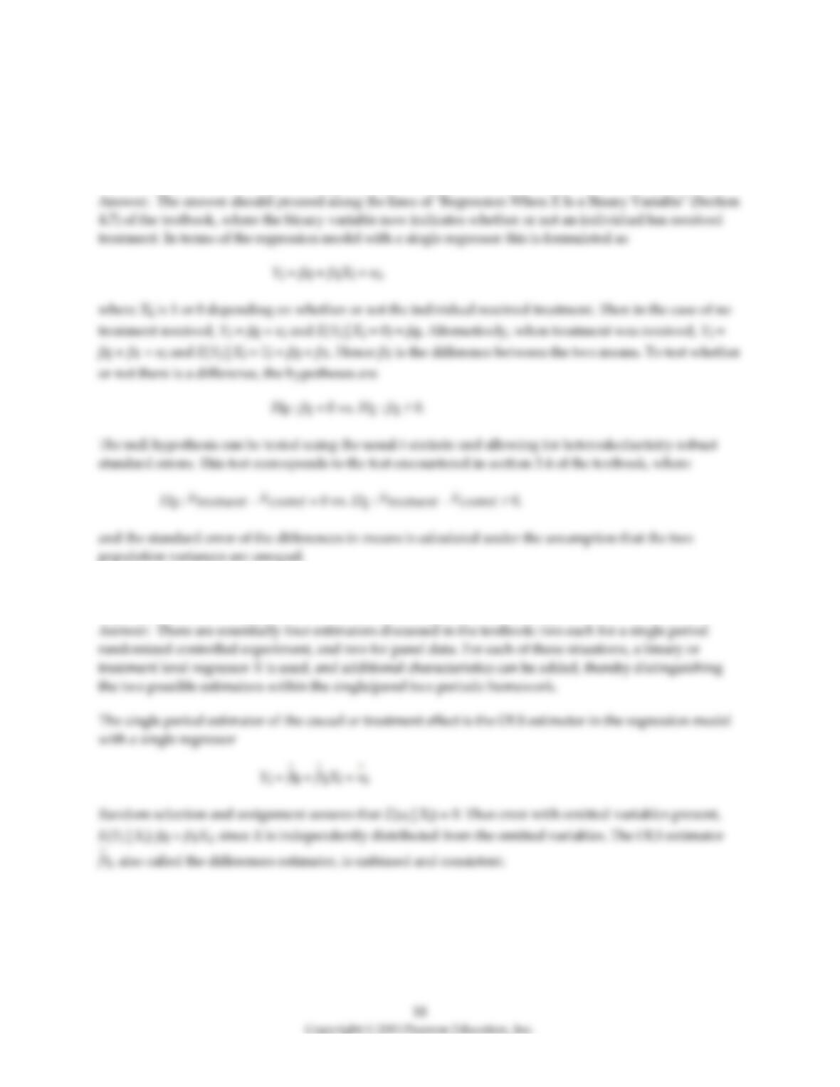
Use a figure similar to the textbook to explain what this reviewer meant.
4) Consider the simple population regression model where the treatment is the same for the members of
the treatment group, and hence X is a binary variable. Explain why the coefficient on X represents the
difference between two means. How is the test for the statistical significance of the coefficient on X
related to the test for differences in means between two populations, when their variances are different?
Write down the null and alternative hypothesis in each case.
5) Present alternative estimators for causal effects using experimental data when data is available for a
single period or for two periods. Discuss their advantages and disadvantages.

6) To analyze the effect of a minimum wage increase, a famous study used a quasi-experiment for two
adjacent states: New Jersey and (Eastern) Pennsylvania. A was calculated by comparing
average employment changes per restaurant between to treatment group (New Jersey) and the control
group (Pennsylvania). In addition, the authors provide data on the employment changes between "low
wage" restaurants and "high wage" restaurants in New Jersey only. A restaurant was classified as "low
wage," if the starting wage in the first wave of surveys was at the then prevailing minimum wage of
$4.25. A "high wage" restaurant was a place with a starting wage close to or above the $5.25 minimum
wage after the increase.
(a) Explain why employment changes of the "high wage" and "low wage" restaurants might constitute a
quasi-experiment. Which is the treatment group and which the control group?
(b) The following information is provided
Low wage
High wage
FTE Employment before
19.56
22.25
FTE Employment after
20.88
20.21
Where FTE is "full time equivalent" and the numbers are average employment per restaurant.
Calculate the change in the treatment group, the change in the control group, and finally .
Since minimum wages represent a price floor, did you expect to be positive or negative?
(c) The standard error for is 1.48. Test whether or not this is statistically significant, given
that there are 174 observations.
7) Specify the multiple regression model that contains the difference-in-difference estimator (with
additional regressors). Explain the circumstances under which this model is preferable to the simple
difference-in-difference estimator. Explain how the W's can be used to test for randomization. How does
the interpretation of the W variables change compared to the differences estimator with additional
regressors?
22
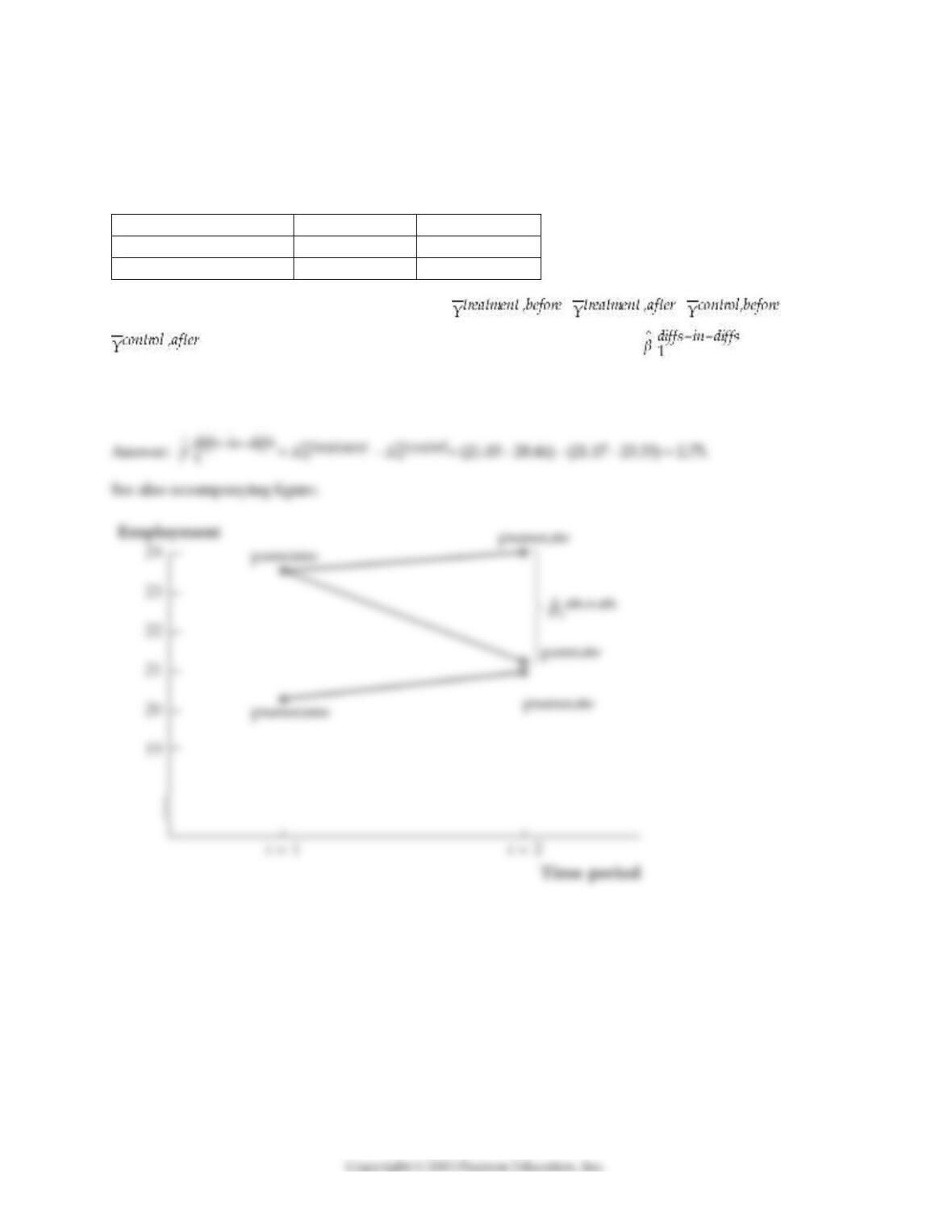
8) Let the vertical axis of a figure indicate the average employment fast food restaurants. There are two
time periods, t = 1 and t = 2, where time period is measured on the horizontal axis. The following table
presents average employment levels per restaurant for New Jersey (the treatment group) and Eastern
Pennsylvania (the control group).
PA
NJ
FTE Employment before
23.33
20.44
FTE Employment after
21.17
21.03
Enter the four points in the figure and label them , , , and
. Connect the points. Finally calculate and indicate the value for .
9) (Requires Appendix material) Discuss how the differences-in-differences estimator can be extended to
multiple time periods. In particular, assume that there are n individuals and T time periods. What do the
individual and time effects control for?
10) The New Jersey-Pennsylvania study on the effect of minimum wages on employment mentioned in
your textbook used a comparison in means "before" and "after" analysis. The difference-in-difference
estimate turned out to be 2.76 with a standard error of 1.36.
The authors also used a difference-in-differences estimator with additional regressors of the type
ΔYi = β0 + β1Xi + β2W1,t + ... + β1+ rWr,i + ui
where i = 1, …, 410. X is a binary variable taking on the value one for the 331 observations in New Jersey.
Since the authors looked at Burger King, KFC, Wendy's, and Roy Rogers fast food restaurants and the
restaurant could be company owned, four W-variables were added.
(a) Given that there are four chains and the possibility of a company ownership, why did the authors not
include five W-variables?
(b) OLS estimation resulted in 1 of 2.30 with a standard error of 1.20. Test for statistical significance and
specify the alternative hypothesis.
(c) Why is this estimate different from the number calculated from Δ – Δ = 2.76? What is
the advantage of employing this estimator of the simple difference-in-difference estimator?


