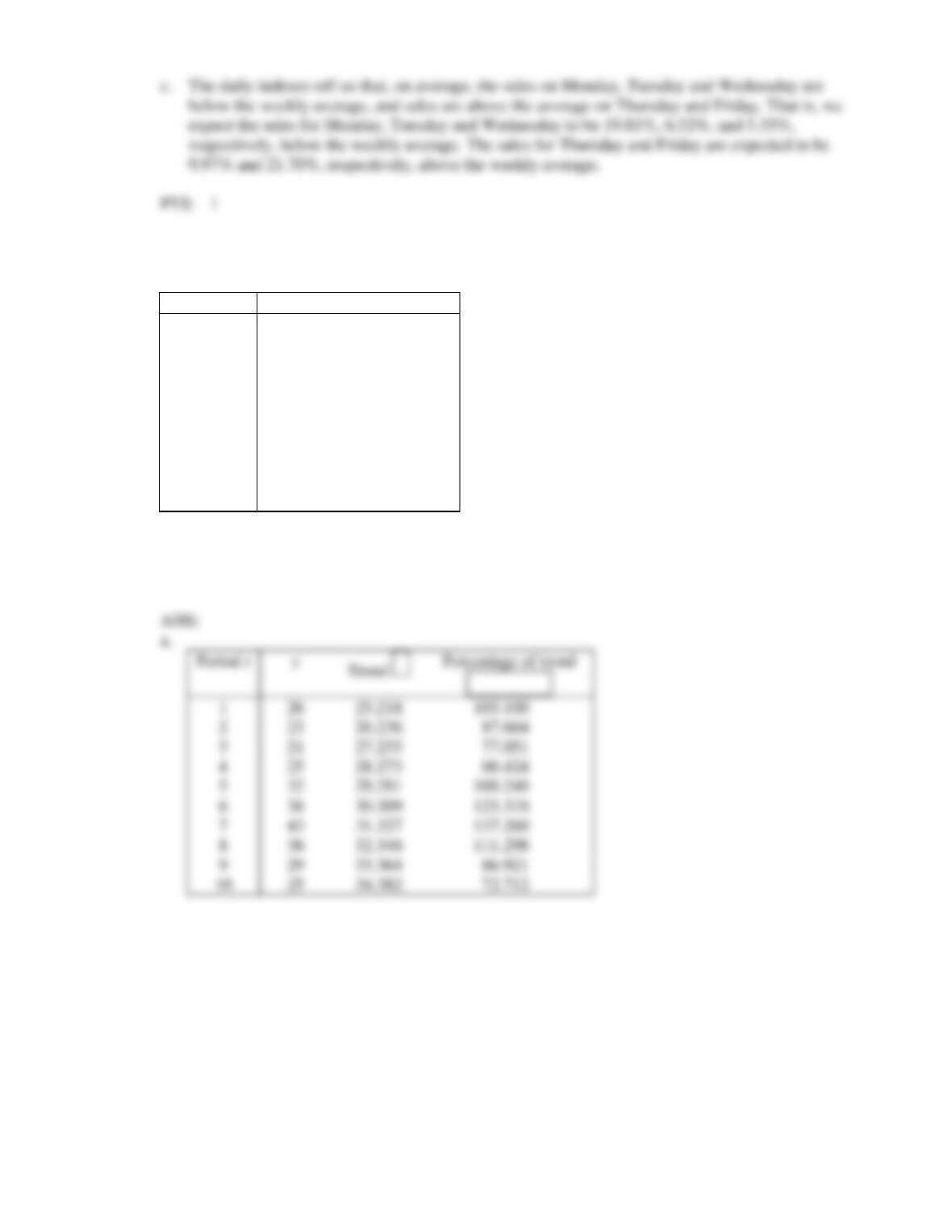
8. Annual production (in millions) of computer chips in a large electronics company was recorded, as
shown below.
Year
t
Production
1990
1
26
1991
2
23
1992
3
21
1993
4
25
1994
5
32
1995
6
38
1996
7
43
1997
8
36
1998
9
29
1999
10
25
a. Calculate the percentage of trend for each time period.
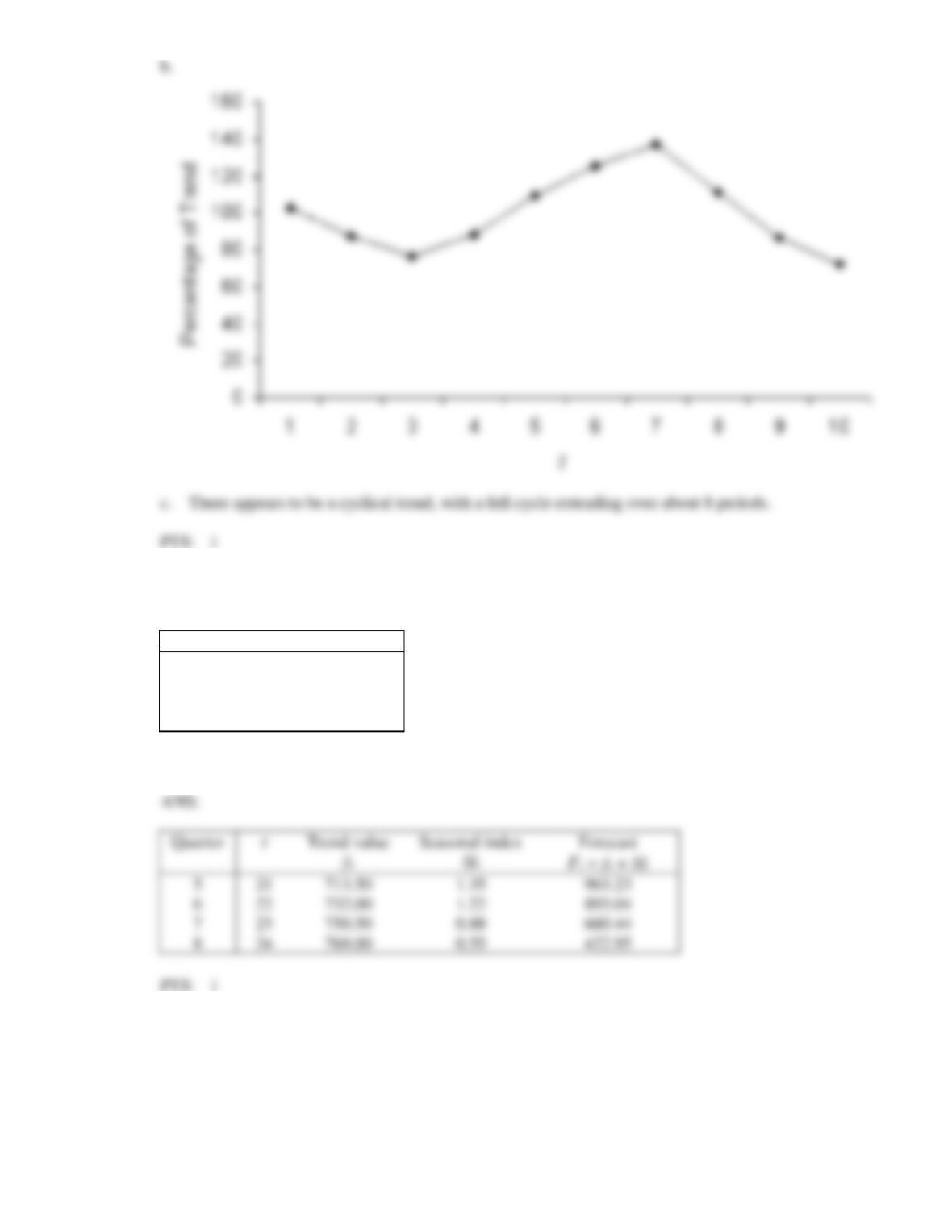
b. Plot the percentage of trend.
c. Describe the cyclical effect (if there is one).
1
2
3
4
5
6
7
8
9
9. The following seasonal indexes and trend line were computed from five years of quarterly sales data.
Trend line: ŷt = 325 + 18.5t, t = 1, 2, 3, …20.
Quarter
Seasonal index
1
1.35
2
1.22
3
0.88
4
0.55
Forecast the sales for the next four quarters.
1.35
0.88
0.55
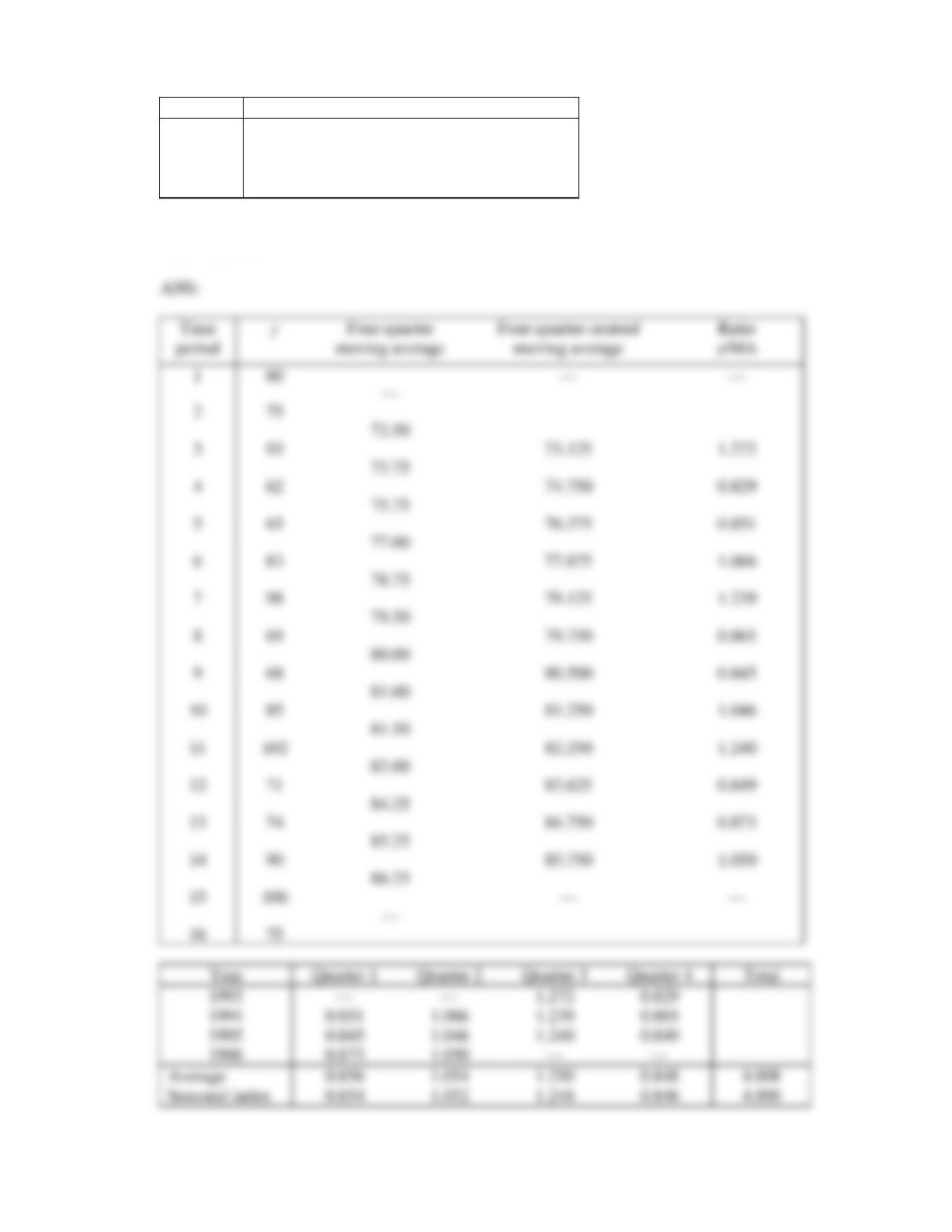
10. The quarterly earnings of a large microcomputer company have been recorded for the years
1993–1996. These data (in millions of dollars) are shown in the accompanying table.
Year
Quarter
1993
1994
1995
1996
1
60
65
68
74
2
75
83
85
90
3
93
98
102
106
4
62
69
71
75
Using an appropriate moving average, measure the quarterly variation by computing the seasonal
(quarterly) indexes.
Total
1.272
0.829
0.851
1.066
1.239
0.865
0.845
1.046
1.240
0.849
0.873
1.050
0.856
1.054
1.250
0.848
11. The trend line
tyt2125
ö+=
and seasonal indexes shown below were computed from 10 years of
quarterly data. Forecast the values for the next four quarters.
Quarter
t
SI
1
0.6
2
1.3
3
1.6
4
0.5
1
2
3
4
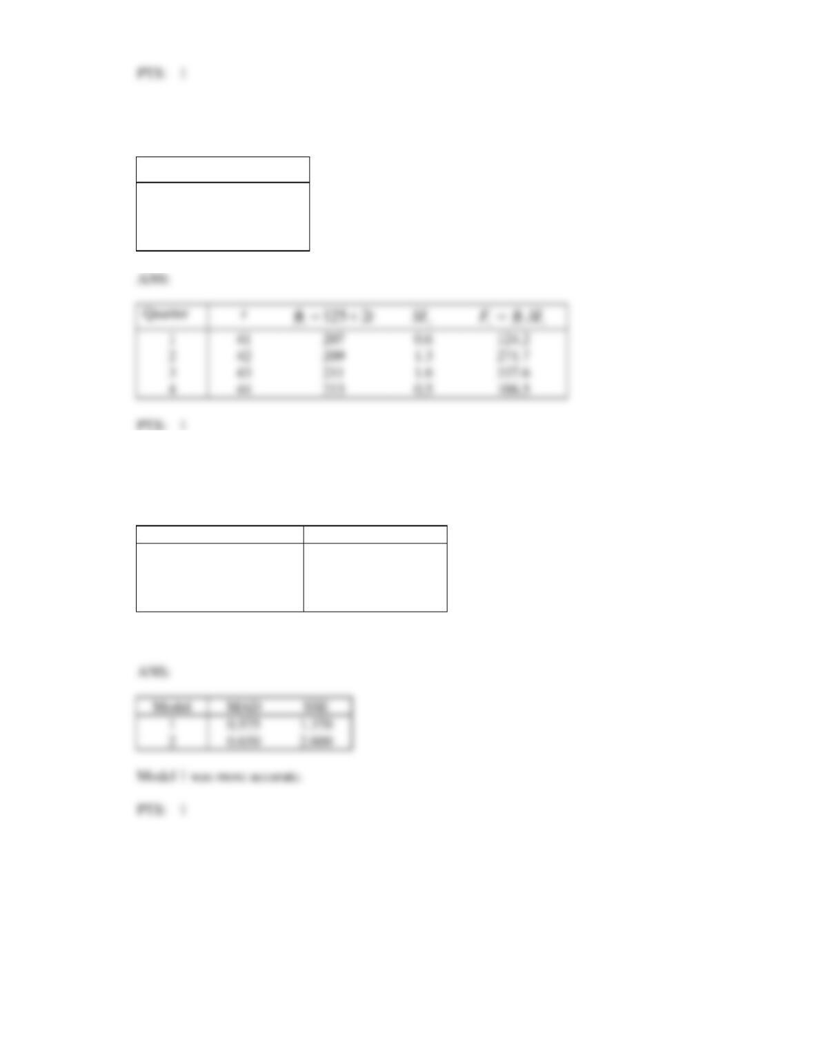
12. Two forecasting models were used to predict the future values of a time series. These are shown in the
following table, together with the actual values.
Forecast Value
t
F
Actual Value
t
y
Model 1
Model 2
8.2
7.7
7.6
7.8
8.5
8.2
7.0
8.5
7.6
9.6
9.0
10.3
Compute MAD and SSE for each model to determine which was more accurate.
1
2
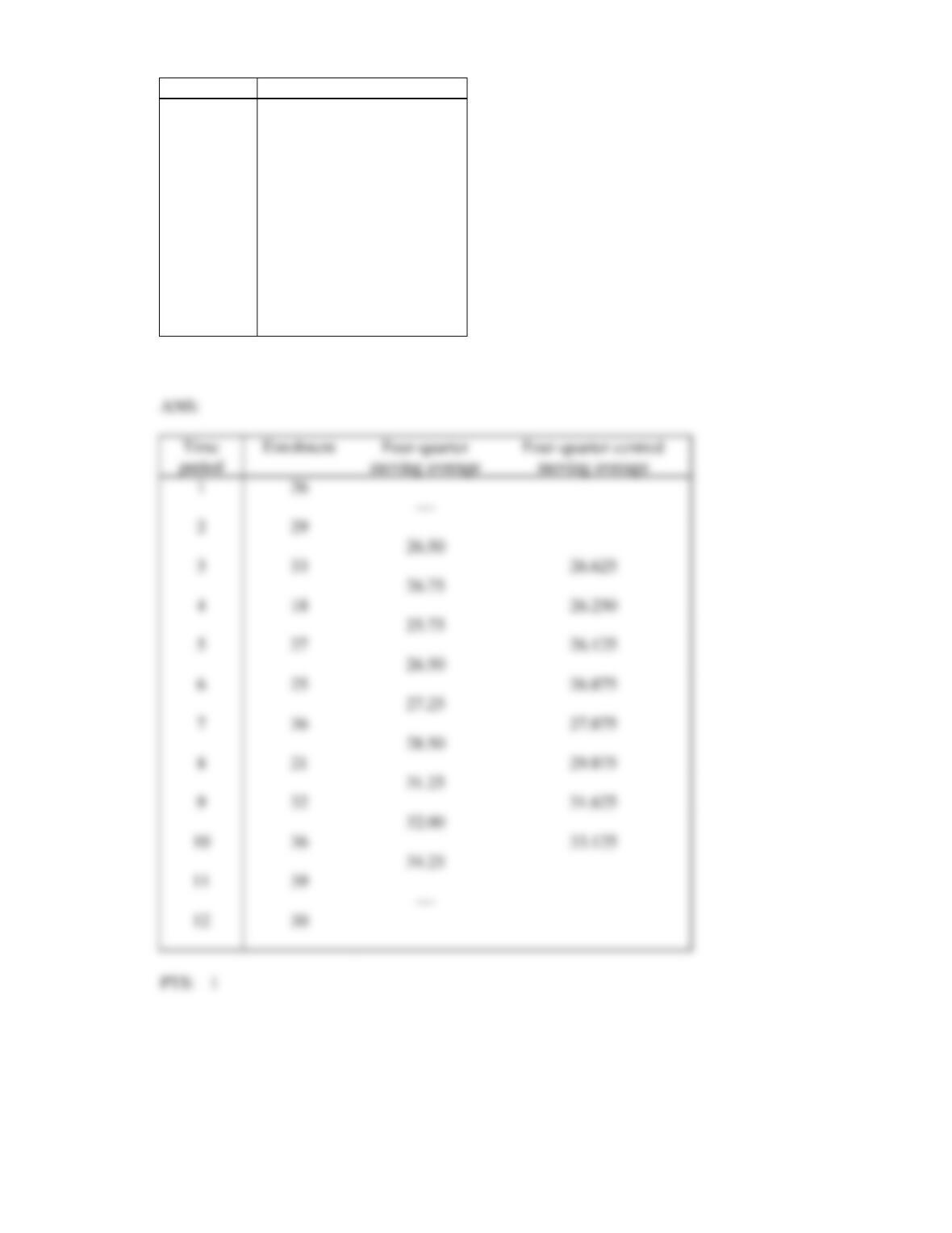
13. Quarterly enrolments in a business statistics class for three years are shown below.
Year
Quarter
Enrolment
1996
1
26
2
29
3
33
4
18
1997
1
27
2
25
3
36
4
21
1998
1
32
2
36
3
39
4
30
Compute the four-quarter centred moving averages.
14. The actual and forecast values of a time series are shown below.
period
Actual values
t
y
Forecast values
t
F
135
140
162
165
155
150
182
191
174
168
194
190
233
220
280
240
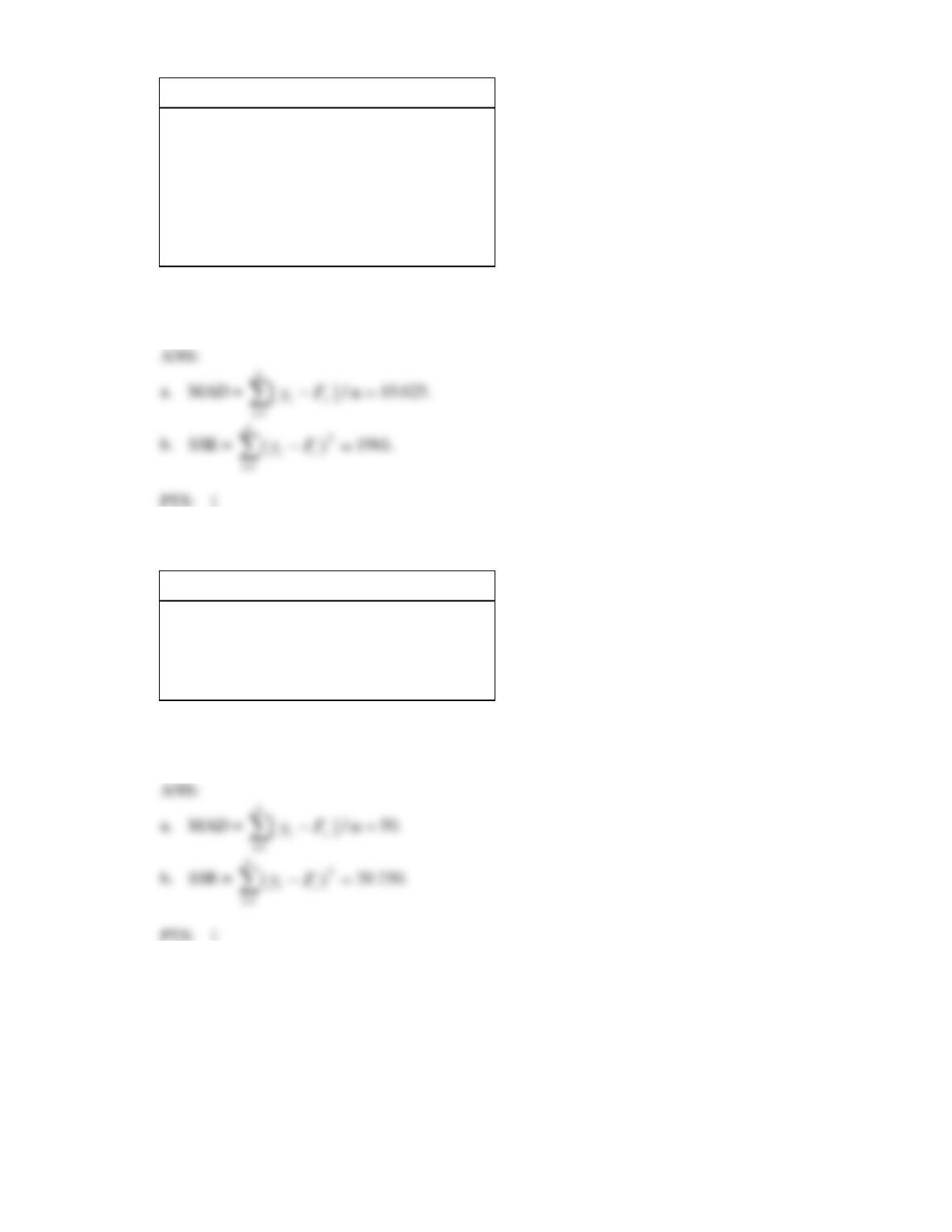
a. Calculate the mean absolute deviation (MAD).
b. Calculate the sum of squares for forecast error (SSE).
15. The actual and forecast values of a time series are shown below.
Actual values
t
y
Forecast values
t
F
2325
2330
2555
2595
2835
2860
3185
3125
3510
3390
a. Calculate the mean absolute deviation (MAD).
b. Calculate the sum of squares for forecast error (SSE).
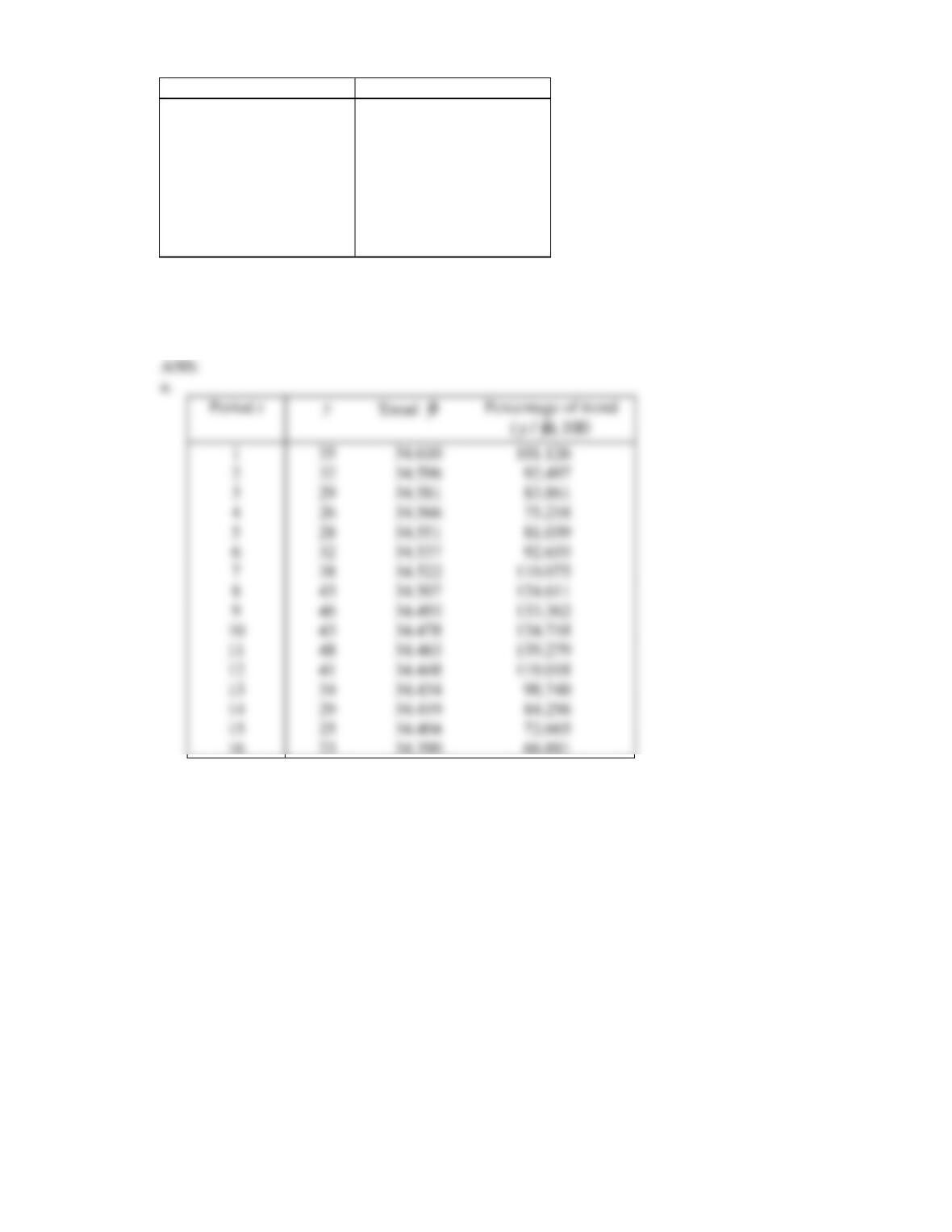
16. Consider the time series shown in the following table.
Time period
y
Time period
y
1
35
9
46
2
32
10
43
3
29
11
48
4
26
12
41
5
28
13
34
6
32
14
29
7
38
15
25
8
43
16
23
a. Calculate the percentage of trend for each time period.
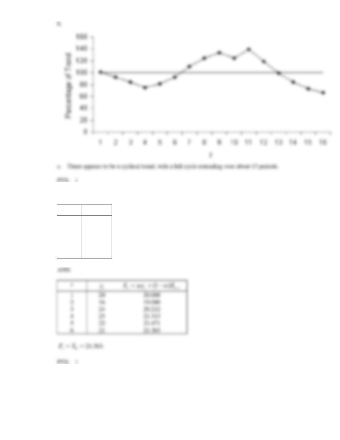
b. Plot the percentage of trend.
c. Describe the cyclical effect (if there is one).
35
32
29
26
28
32
38
43
46
43
48
41
34
29
25
23
17. Use exponential smoothing, with w = 0.23 to forecast the next value of the time series below.
t
t
y
1
20
2
16
3
24
4
25
5
22
6
21
t
y
20
16
24
25
21
18. Regression analysis with t = 1 to 40 was used to develop the following equation:
321 0.38.15.151500
öQQQtyt−+++=
,
where:
i
Q
= 1, if quarter i (i = 1, 2, 3)
= 0, otherwise.
Forecast the next four quarters.
19. The quarterly sales (in millions of dollars) of a department store chain were recorded for the years
1995–1998. They are listed below.
Year
Quarter
Sales
1995
1
21
2
36
3
28
4
44
1996
1
25
2
23
3
39
4
36
1997
1
30
2
41
3
47
4
55
1998
1
34
2
29
3
32
4
48
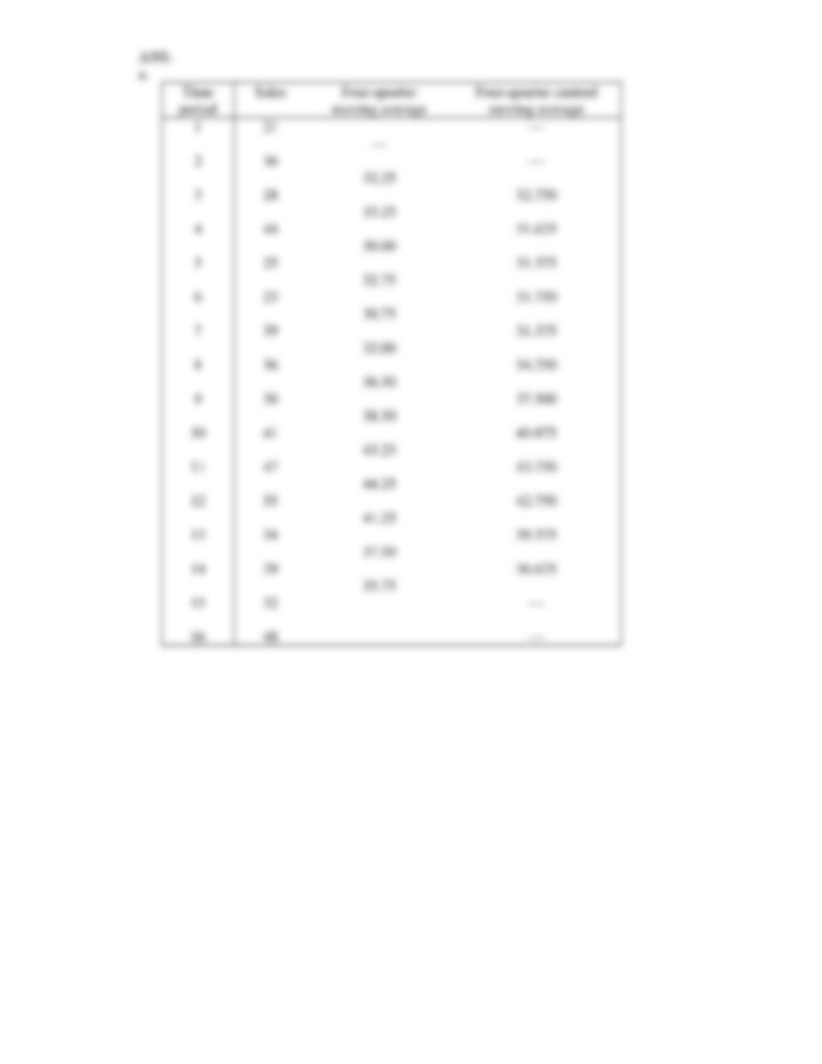
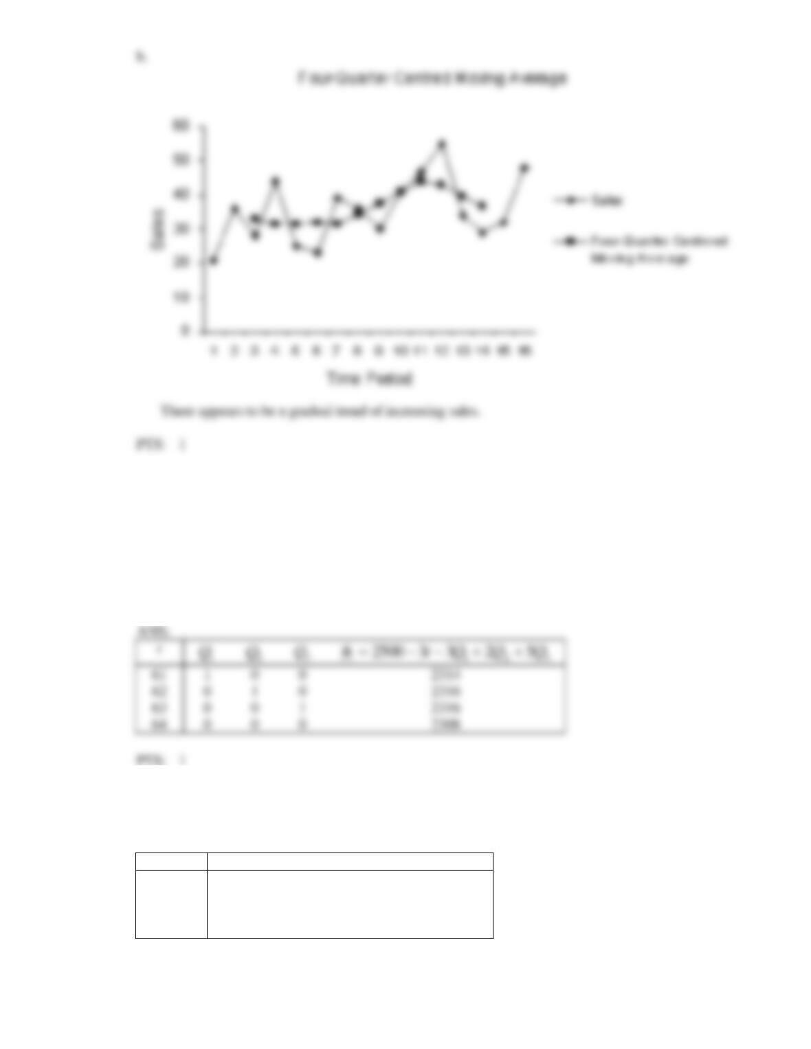
a. Calculate the four-quarter centred moving averages.
b. Graph the time series and the moving averages. What can you conclude from your time-series
smoothing?
0
1
0
0
0
1
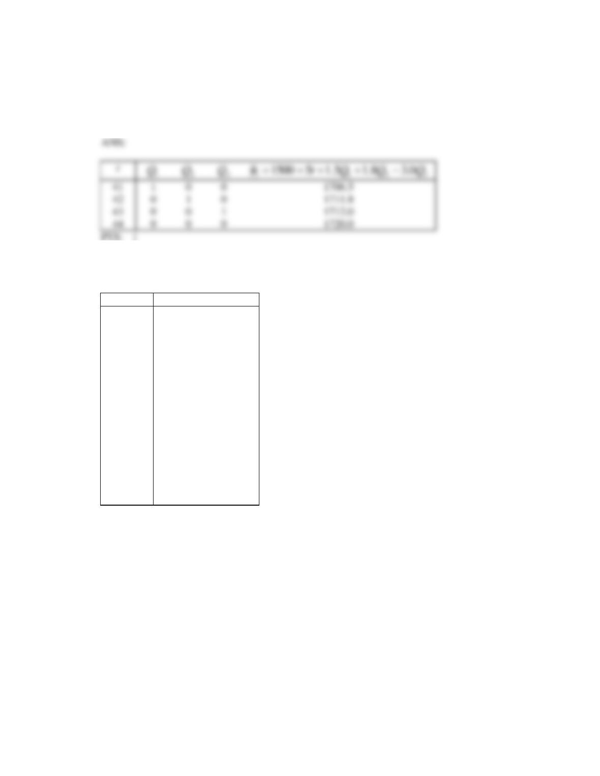
20. Regression analysis was used to develop the following equation from 60 observations of quarterly
data:
321 52332500
öQQQtyt++−−=
,
where:
i
Q
= 1, if quarter i (i = 1, 2, 3)
= 0, otherwise
Forecast the next four quarters.
321 52332500
öQQQtyt++−−=
21. The number of pairs of sunglasses sold each quarter in a beachside drugstore were recorded for the
years 2007–2010. These data are shown in the following table.
Year
Quarter
2007
2008
2009
2010
1
82
84
85
90
2
72
71
70
74
3
65
66
67
71
4
53
54
56
58

a. Develop a regression model, using indicator variables to represent quarters.
b. Forecast the quarterly earnings for the years 2011 and 2012.
22. Regression analysis with t = 1 to 80 was used to develop the following forecast equation:
ŷt = 135 + 4.8t − 1.3Q1 − 1.7Q2 + 1.5Q3
where:
Qi = 1, if quarter i (i = 1, 2, 3)
= 0, otherwise.
Forecast the next four values.
23. A local newspaper that appears six days per week wanted to forecast two-day revenues from its
business services classified ads section. The revenues (in $1000s) were recorded for the past 52 weeks.
From these data, the following regression equation was computed:
21 401506.02000
öDDtyt−−+=
, t = 1, 2, 3,…156,
where:
1
D
= 1, if Monday or Tuesday
= 0, otherwise.
2
D
= 1, if Wednesday or Thursday
= 0, otherwise.
Forecast the two-day revenues for the next week.
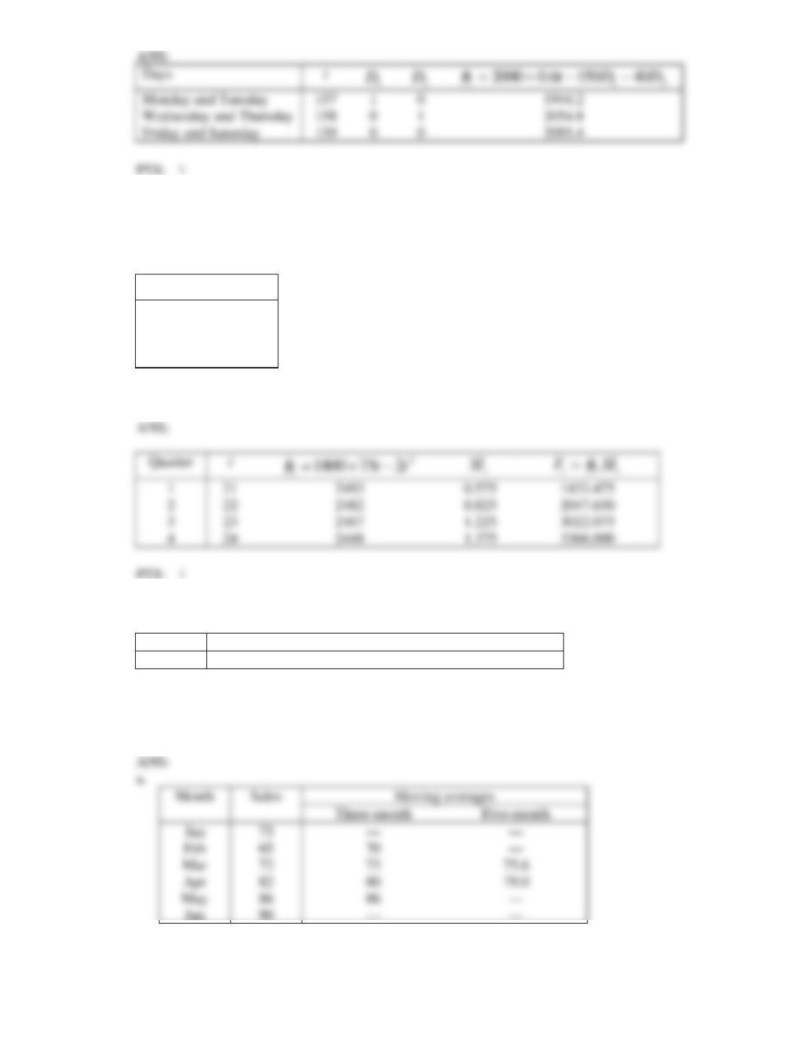
24. The following trend line and seasonal indexes were computed from five years of quarterly
observations:
2
2751800
öttyt−+=
.
Quarter
t
SI
1
0.575
2
0.825
3
1.225
4
1.375
Forecast the four quarterly values for next year.
t
SI
1
0.575
2
0.825
3
1.225
4
1.375
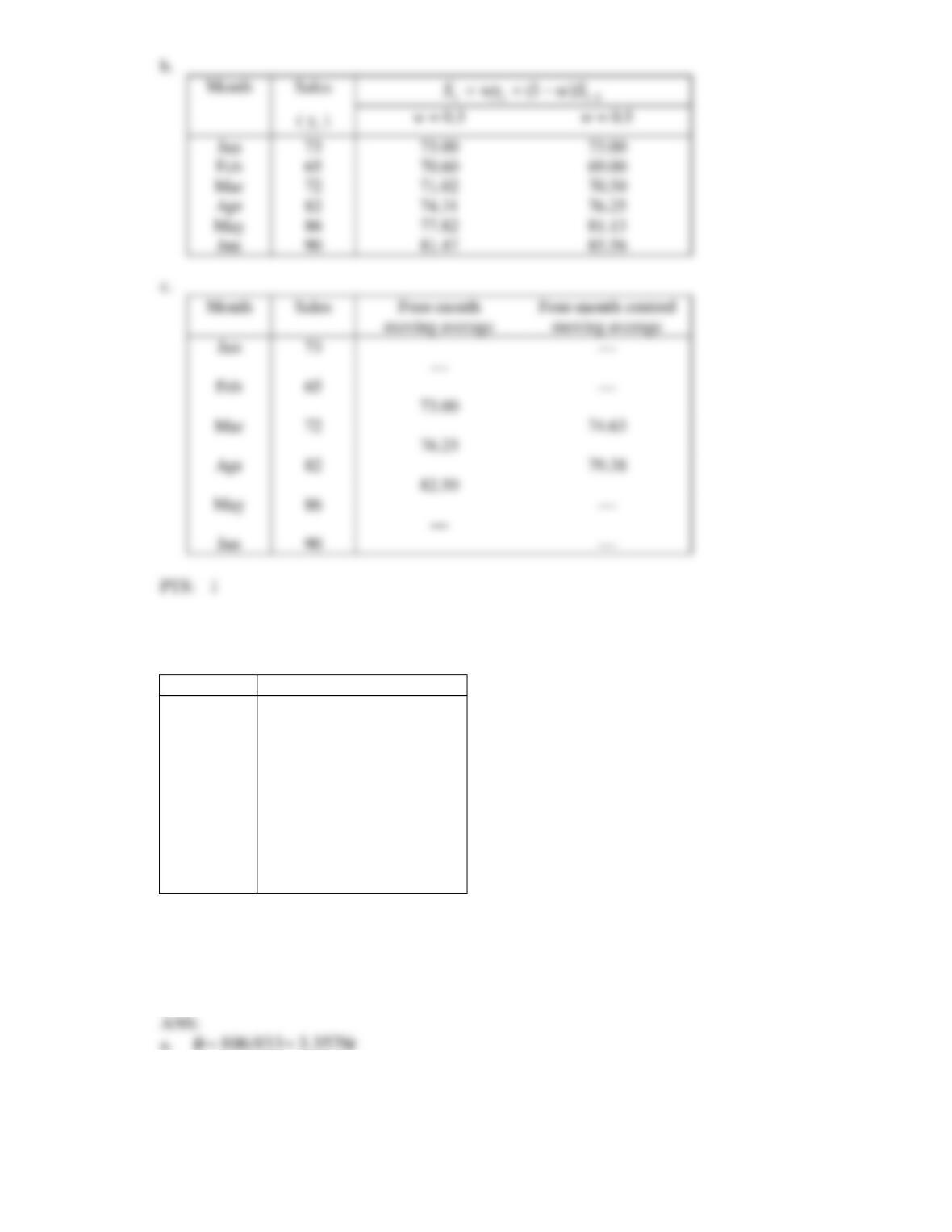
25. Monthly sales (in $1000s) of a computer store are shown below.
Month
Jan
Feb
Mar
Apr
May
Jun
Sales
73
65
72
82
86
90
a. Compute the three-month and five-month moving averages.
b. Compute the exponentially smoothed sales with w = 0.3 and w = 0.5
c. Calculate the four-month moving average, and four-month centred moving average.
Sales
Monday and Tuesday
1
0
Wednesday and Thursday
Friday and Saturday
0
0
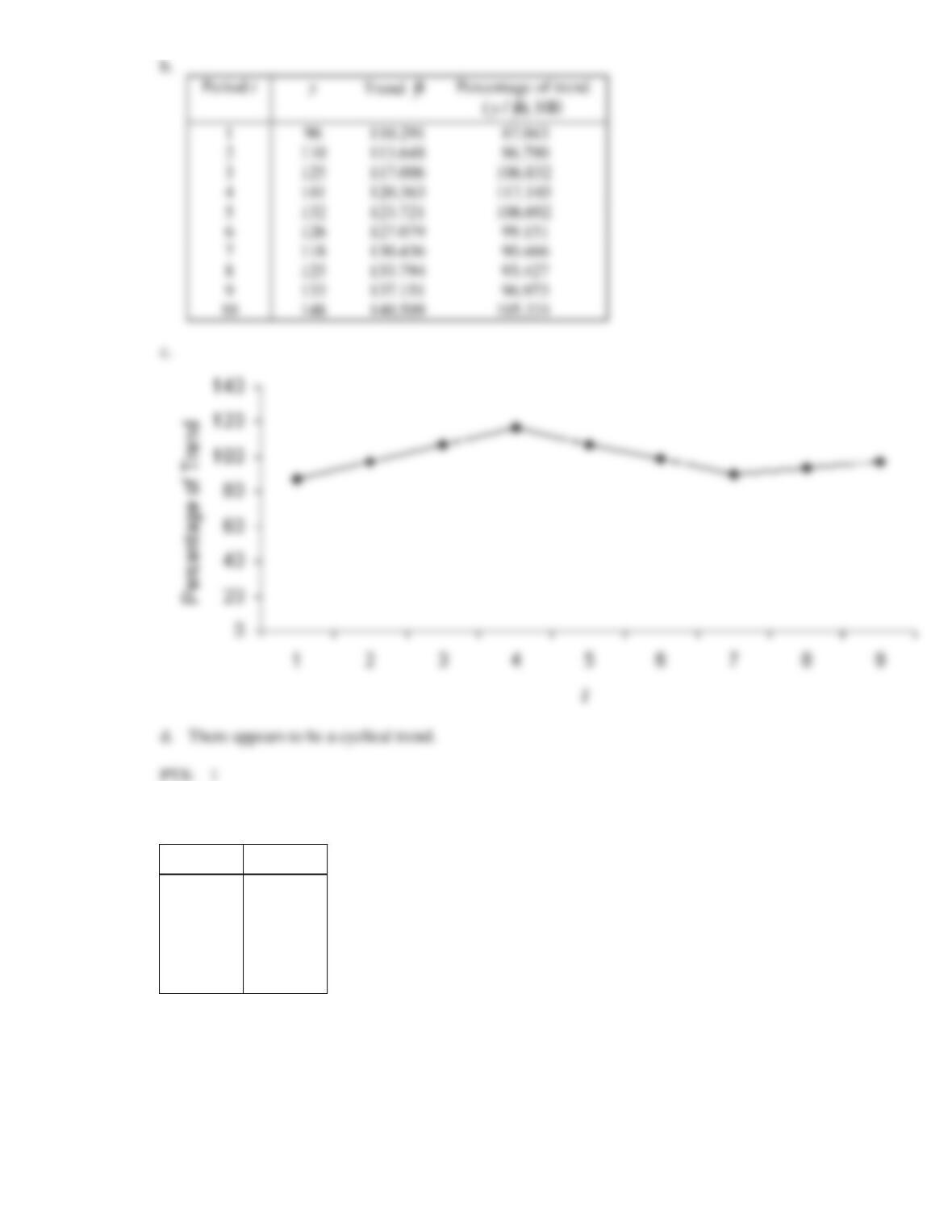
26. The agricultural exports (in millions of dollars) from a Latin American country for 10 years are shown
below.
Year
t
Exports
1988
1
96
1989
2
110
1990
3
125
1991
4
141
1992
5
132
1993
6
126
1994
7
118
1995
8
125
1996
9
133
1997
10
148
a. Use the regression technique to calculate the linear trend line.
b. Calculate the percentage of trend.
c. Plot the percentage of trend.
d. Describe the cyclical effect (if there is one).
.
27. A time series for the years 1990–1995 is shown below.
Year
t
y
1990
125
1991
115
1992
120
1993
126
1994
140
1995
122
a. Develop forecasts for the years 1996–1998, with the following smoothing constant values:
w = 0.2, w = 0.5 and w = 0.6.
b. Compare each of the three sets of forecasts above with the actual values for 1996–1998 given in
the following table, and compute the MAD for each model. Which model is best?
110
125
141
132
126
118
125
133
148