Day
Precipitation
Number of accidents
1
0.05
5
2
0.12
6
3
0.05
2
4
0.08
4
5
0.10
8
6
0.35
14
7
0.15
7
8
0.30
13
9
0.10
7
10
0.20
10
Do these data allow us to conclude at the 10% significance level that the amount of precipitation and
the number of accidents are linearly related?
92. A statistician investigating the relationship between the amount of precipitation (in inches) and the
number of car accidents gathered data for 10 randomly selected days. The results are presented below.
Day
Precipitation
Number of accidents
1
0.05
5
2
0.12
6
3
0.05
2
4
0.08
4
5
0.10
8
6
0.35
14
7
0.15
7
8
0.30
13
9
0.10
7
10
0.20
10
Predict with 95% confidence the number of accidents that occur when there is 0.40 inches of rain.
93. A statistician investigating the relationship between the amount of precipitation (in inches) and the
number of car accidents gathered data for 10 randomly selected days. The results are presented below.
Day
Precipitation
Number of accidents
1
0.05
5
2
0.12
6
3
0.05
2
4
0.08
4
5
0.10
8
6
0.35
14
7
0.15
7
8
0.30
13
9
0.10
7
10
0.20
10
Estimate with 95% confidence the mean daily number of accidents when the daily precipitation is 0.25
inches.
94. A statistician investigating the relationship between the amount of precipitation (in inches) and the
number of car accidents gathered data for 10 randomly selected days. The results are presented below.
Day
Precipitation
Number of accidents
1
0.05
5
2
0.12
6
3
0.05
2
4
0.08
4
5
0.10
8
6
0.35
14
7
0.15
7
8
0.30
13
9
0.10
7
10
0.20
10
Calculate the Spearman rank correlation coefficient, and test to determine at the 5% significance level
whether we can infer that a linear relationship exists between the number of accidents and the amount
of precipitation.
95. At a recent Willie Nelson concert, a survey was conducted that asked a random sample of 20 people
their age and how many concerts they have attended since the beginning of the year. The following
data were collected.
Age
62
57
40
49
67
54
43
65
54
41
Number of concerts
6
5
4
3
5
5
2
6
3
1
Age
44
48
55
60
59
63
69
40
38
52
Number of Concerts
3
2
4
5
4
5
4
2
1
3
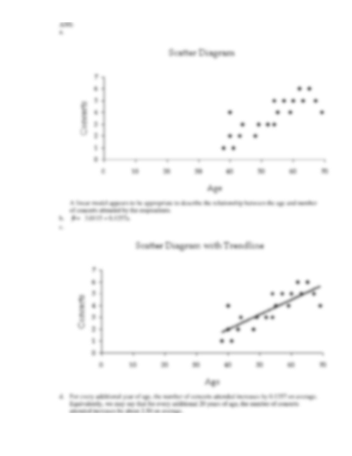
a. Draw a scatter diagram of the data to determine whether a linear model appears to be appropriate
to describe the relationship between the age and number of concerts attended by the respondents.
b. Determine the least squares regression line.
c. Plot the least squares regression line.
d. Interpret the value of the slope of the regression line.
96. At a recent Willie Nelson concert, a survey was conducted that asked a random sample of 20 people
their age and how many concerts they have attended since the beginning of the year. The following
data were collected.
Age
62
57
40
49
67
54
43
65
54
41
Number of concerts
6
5
4
3
5
5
2
6
3
1
Age
44
48
55
60
59
63
69
40
38
52
Number of Concerts
3
2
4
5
4
5
4
2
1
3
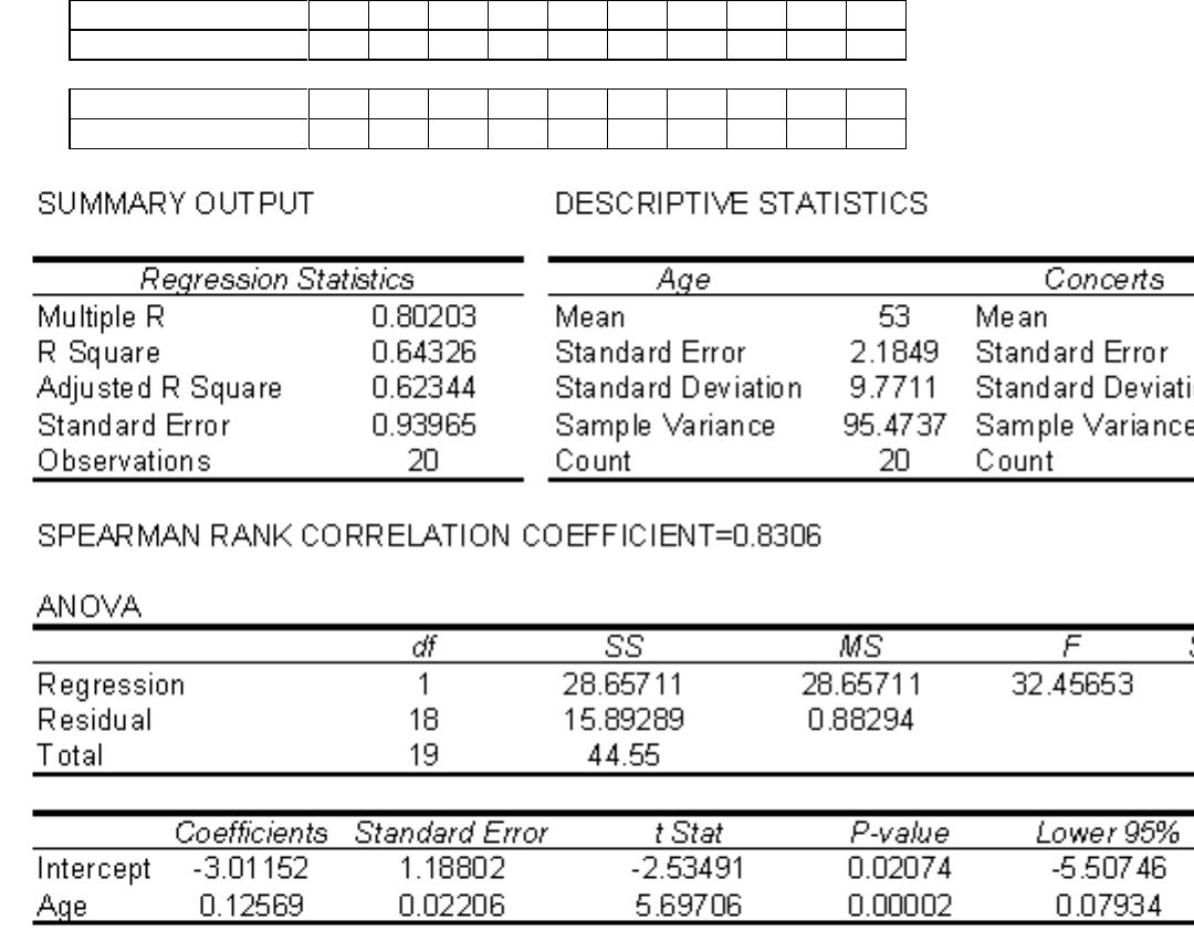
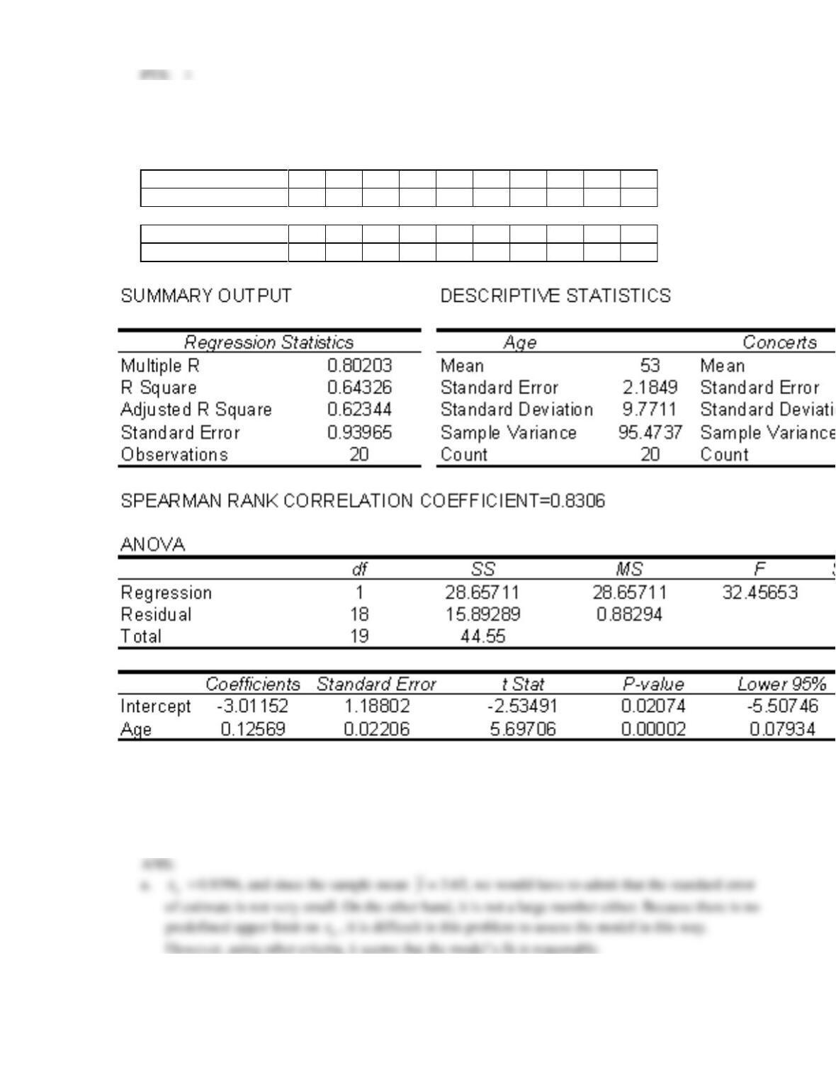
a. Determine the standard error of estimate and describe what this statistic tells you about the
model’s fit.
b. Determine the coefficient of determination, and discuss what its value tells you about the two
variables.
97. At a recent Willie Nelson concert, a survey was conducted that asked a random sample of 20 people
their age and how many concerts they have attended since the beginning of the year. The following
data were collected.
Age
62
57
40
49
67
54
43
65
54
41
Number of concerts
6
5
4
3
5
5
2
6
3
1
Age
44
48
55
60
59
63
69
40
38
52
Number of Concerts
3
2
4
5
4
5
4
2
1
3
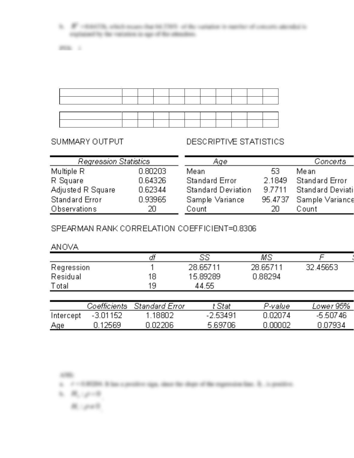
a. Calculate the Pearson correlation coefficient. What sign does it have? Why?
b. Conduct a test of the population coefficient of correlation to determine at the 5% significance level
whether a linear relationship exists between age and number of concerts attended.
98. At a recent Willie Nelson concert, a survey was conducted that asked a random sample of 20 people
their age and how many concerts they have attended since the beginning of the year. The following
data were collected.
Age
62
57
40
49
67
54
43
65
54
41
Number of concerts
6
5
4
3
5
5
2
6
3
1
Age
44
48
55
60
59
63
69
40
38
52
Number of Concerts
3
2
4
5
4
5
4
2
1
3
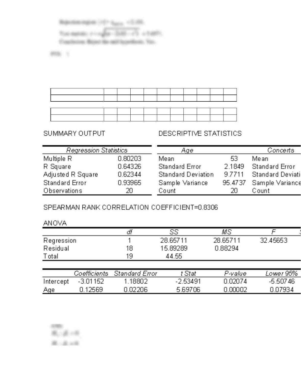
Conduct a test of the population slope to determine at the 5% significance level whether a linear
relationship exists between age and number of concerts attended.
.
99. At a recent Willie Nelson concert, a survey was conducted that asked a random sample of 20 people
their age and how many concerts they have attended since the beginning of the year. The following
data were collected.
Age
62
57
40
49
67
54
43
65
54
41
Number of concerts
6
5
4
3
5
5
2
6
3
1
Age
44
48
55
60
59
63
69
40
38
52
Number of Concerts
3
2
4
5
4
5
4
2
1
3
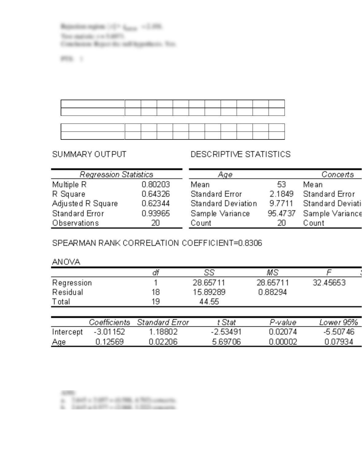
a. Predict with 95% confidence the number of concerts attended by a 45-year-old individual.
b. Predict with 95% confidence the average number of concerts attended by all 45-year-old
individuals.
100. At a recent Willie Nelson concert, a survey was conducted that asked a random sample of 20 people
their age and how many concerts they have attended since the beginning of the year. The following
data were collected.
Age
62
57
40
49
67
54
43
65
54
41
Number of concerts
6
5
4
3
5
5
2
6
3
1
Age
44
48
55
60
59
63
69
40
38
52
Number of Concerts
3
2
4
5
4
5
4
2
1
3
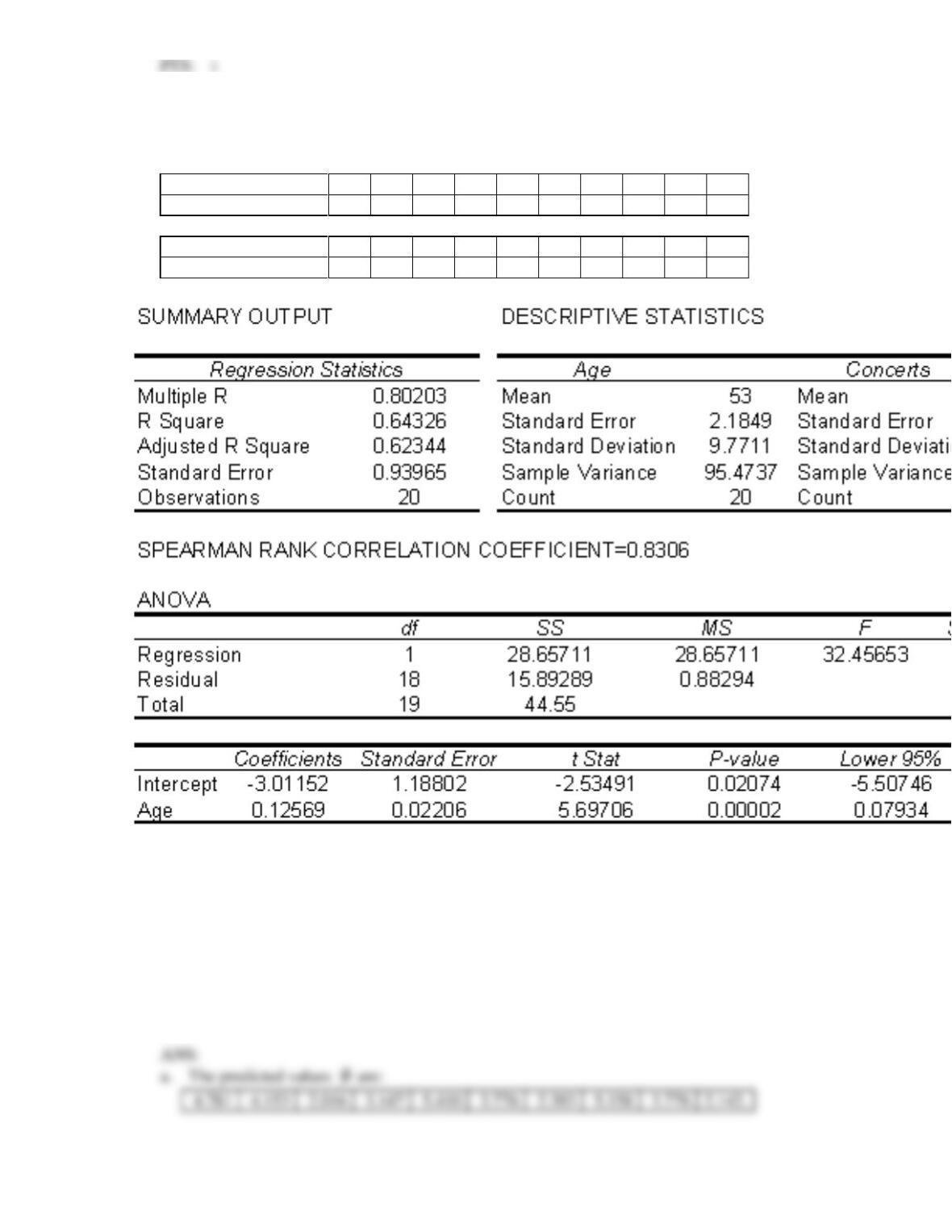
a. Use the regression equation
=y
ö
–3.0115 + 0.1257x to determine the predicted values of y.
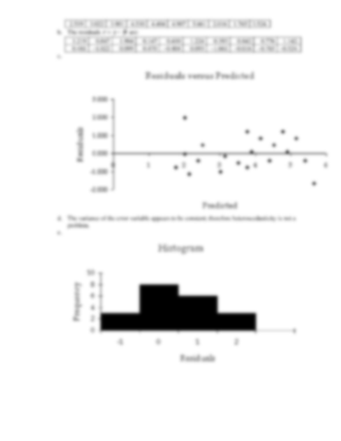
b. Use the predicted values and the actual values of y to calculate the residuals.
c. Plot the residuals against the predicted values
ö
y
.
d. Does it appear that heteroscedasticity is a problem? Explain.
e. Draw a histogram of the residuals.
f. Does it appear that the errors are normally distributed? Explain.
g. Use the residuals to compute the standardised residuals.
h. Identify possible outliers.
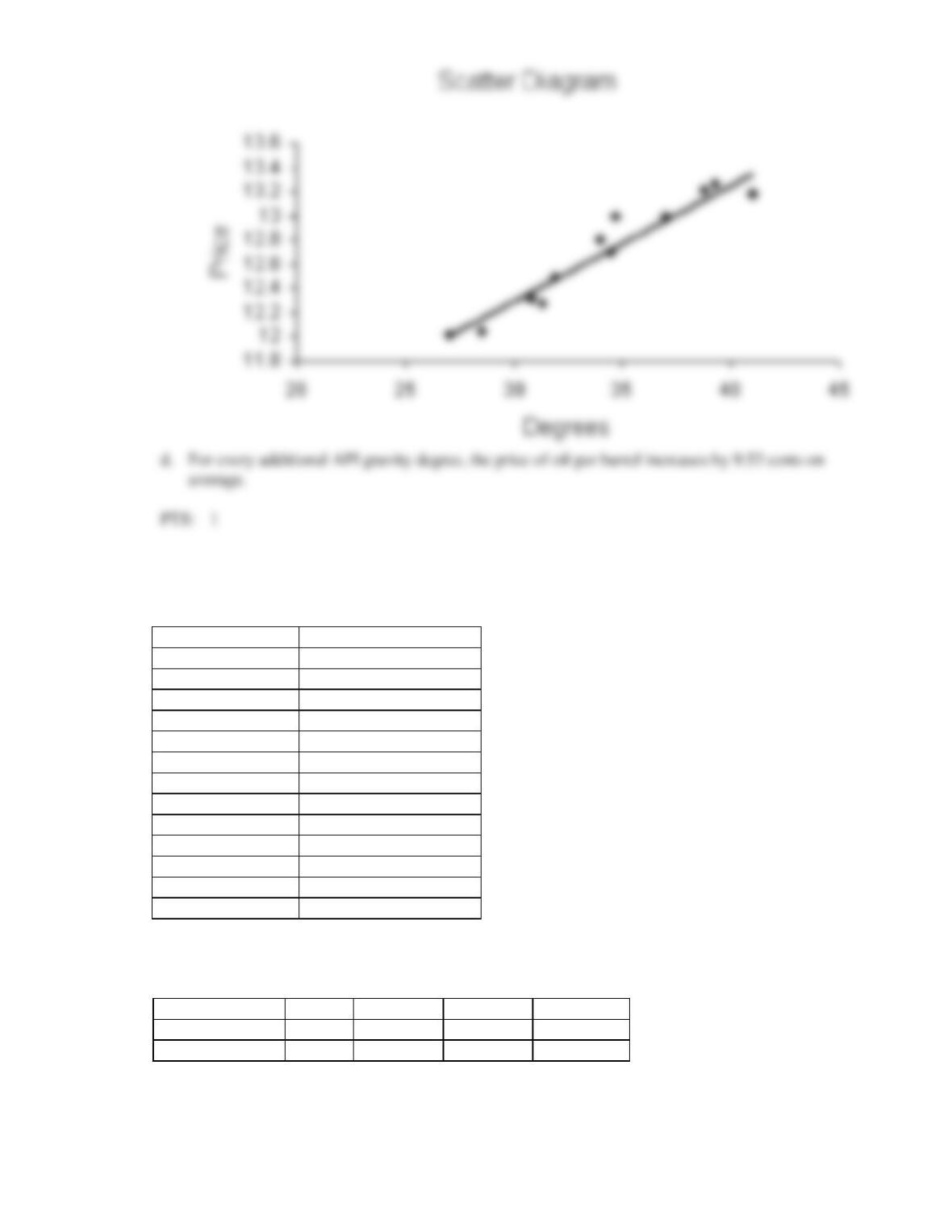
101. The quality of oil is measured in API gravity degrees – the higher the degrees API, the higher the
quality. The table shown below is produced by an expert in the field, who believes that there is a
relationship between quality and price per barrel.
Oil degrees API
Price per barrel (in $)
27.0
12.02
28.5
12.04
30.8
12.32
31.3
12.27
31.9
12.49
34.5
12.70
34.0
12.80
34.7
13.00
37.0
13.00
41.0
13.17
41.0
13.19
38.8
13.22
39.3
13.27
A partial Minitab output follows.
Descriptive Statistics
Variable
N
Mean
StDev
SE Mean
Degrees
13
34.60
4.613
1.280
Price
13
12.730
0.457
0.127
Covariances
Degrees
Price
Degrees
21.281667
Price
2.026750
0.208833
Regression Analysis
Predictor
Coef
StDev
T
P
Constant
9.4349
0.2867
32.91
0.000
Degrees
0.095235
0.008220
11.59
0.000
S = 0.1314 R-Sq = 92.46% R-Sq(adj) = 91.7%
1.297
0.902
2.111
1.303
0.896
Analysis of Variance
Source
DF
SS
MS
F
P
Regression
1
2.3162
2.3162
134.24
0.000
Residual Error
11
0.1898
0.0173
Total
12
2.5060
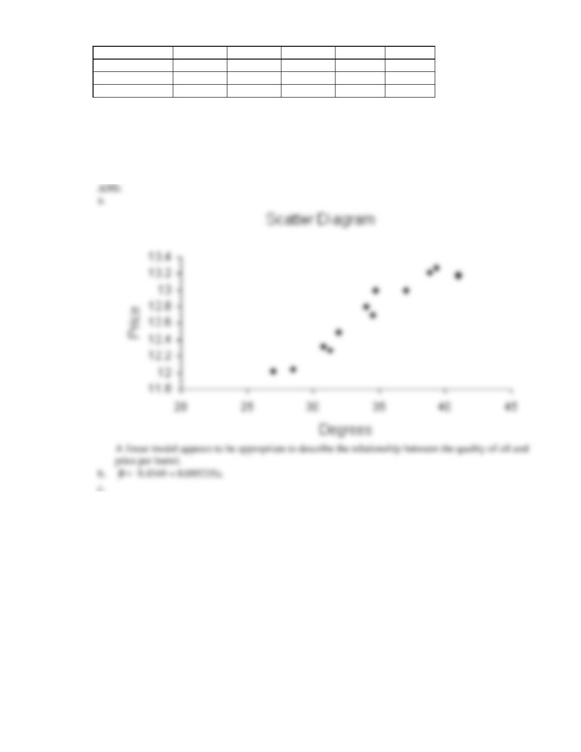
a. Draw a scatter diagram of the data to determine whether a linear model appears to be appropriate
to describe the relationship between the quality of oil and price per barrel.
b. Determine the least squares regression line.
c. Redraw the scatter diagram and plot the least squares regression line on it.
d. Interpret the value of the slope of the regression line.
102. The quality of oil is measured in API gravity degrees – the higher the degrees API, the higher the
quality. The table shown below is produced by an expert in the field, who believes that there is a
relationship between quality and price per barrel.
Oil degrees API
Price per barrel (in $)
27.0
12.02
28.5
12.04
30.8
12.32
31.3
12.27
31.9
12.49
34.5
12.70
34.0
12.80
34.7
13.00
37.0
13.00
41.0
13.17
41.0
13.19
38.8
13.22
39.3
13.27
A partial Minitab output follows.
Descriptive Statistics
Variable
N
Mean
StDev
SE Mean
Degrees
13
34.60
4.613
1.280
Price
13
12.730
0.457
0.127
Covariances
Degrees
Price
Degrees
21.281667
Price
2.026750
0.208833
Regression Analysis
Predictor
Coef
StDev
T
P
Constant
9.4349
0.2867
32.91
0.000
Degrees
0.095235
0.008220
11.59
0.000
S = 0.1314 R-Sq = 92.46% R-Sq(adj) = 91.7%
Analysis of Variance
Source
DF
SS
MS
F
P
Regression
1
2.3162
2.3162
134.24
0.000
Residual Error
11
0.1898
0.0173
Total
12
2.5060
a. Determine the standard error of estimate and describe what this statistic tells you.
b. Determine the coefficient of determination and discuss what its value tells you about the two
variables.
c. Calculate the Pearson correlation coefficient. What sign does it have? Why?
103. The quality of oil is measured in API gravity degrees – the higher the degrees API, the higher the
quality. The table shown below is produced by an expert in the field, who believes that there is a
relationship between quality and price per barrel.
Oil degrees API
Price per barrel (in $)
27.0
12.02
28.5
12.04
30.8
12.32
31.3
12.27
31.9
12.49
34.5
12.70
34.0
12.80
34.7
13.00
37.0
13.00
41.0
13.17
41.0
13.19
38.8
13.22
39.3
13.27
A partial Minitab output follows.
Descriptive Statistics
Variable
N
Mean
StDev
SE Mean
Degrees
13
34.60
4.613
1.280
Price
13
12.730
0.457
0.127
Covariances
Degrees
Price
Degrees
21.281667
Price
2.026750
0.208833
Regression Analysis
Predictor
Coef
StDev
T
P
Constant
9.4349
0.2867
32.91
0.000
Degrees
0.095235
0.008220
11.59
0.000
S = 0.1314 R-Sq = 92.46% R-Sq(adj) = 91.7%
Analysis of Variance
Source
DF
SS
MS
F
P
Regression
1
2.3162
2.3162
134.24
0.000
Residual Error
11
0.1898
0.0173
Total
12
2.5060
Conduct a test of the population coefficient of correlation to determine at the 5% significance level
whether a linear relationship exists between the quality of oil and price per barrel.
104. The quality of oil is measured in API gravity degrees – the higher the degrees API, the higher the
quality. The table shown below is produced by an expert in the field, who believes that there is a
relationship between quality and price per barrel.
Oil degrees API
Price per barrel (in $)
27.0
12.02
28.5
12.04
30.8
12.32
31.3
12.27
31.9
12.49
34.5
12.70
34.0
12.80
34.7
13.00
37.0
13.00
41.0
13.17
41.0
13.19
38.8
13.22
39.3
13.27
A partial Minitab output follows.
Descriptive Statistics
Variable
N
Mean
StDev
SE Mean
Degrees
13
34.60
4.613
1.280
Price
13
12.730
0.457
0.127
Covariances
Degrees
Price
Degrees
21.281667
Price
2.026750
0.208833
Regression Analysis
Predictor
Coef
StDev
T
P
Constant
9.4349
0.2867
32.91
0.000
Degrees
0.095235
0.008220
11.59
0.000
S = 0.1314 R-Sq = 92.46% R-Sq(adj) = 91.7%
Analysis of Variance
Source
DF
SS
MS
F
P
Regression
1
2.3162
2.3162
134.24
0.000
Residual Error
11
0.1898
0.0173
Total
12
2.5060
Conduct a test of the population slope to determine at the 5% significance level whether a linear
relationship exists between the quality of oil and price per barrel.