Unlock document.
This document is partially blurred.
Unlock all pages and 1 million more documents.
Get Access

PTS: 1
57. An ardent fan of television game shows has observed that, in general, the more educated the
contestant, the less money he or she wins. To test her belief, she gathers data about the last eight
winners of her favourite game show. She records their winnings in dollars and their years of education.
The results are as follows.
Contestant
Years of
education
Winnings
1
11
750
2
15
400
3
12
600
4
16
350
5
11
800
6
16
300
7
13
650
8
14
400
Predict with 95% confidence the winnings of a contestant who has 15 years of education.
58. An ardent fan of television game shows has observed that, in general, the more educated the
contestant, the less money he or she wins. To test her belief, she gathers data about the last eight
winners of her favourite game show. She records their winnings in dollars and their years of education.
The results are as follows.
Contestant
Years of
education
Winnings
1
11
750
2
15
400
3
12
600
4
16
350
5
11
800
6
16
300
7
13
650
8
14
400
Predict with 95% confidence the winnings of a contestant who has 10 years of education.

59. An ardent fan of television game shows has observed that, in general, the more educated the
contestant, the less money he or she wins. To test her belief, she gathers data about the last eight
winners of her favourite game show. She records their winnings in dollars and their years of education.
The results are as follows.
Contestant
Years of
education
Winnings
1
11
750
2
15
400
3
12
600
4
16
350
5
11
800
6
16
300
7
13
650
8
14
400
Predict with 95% the winnings of all contestants who have 15 years of education.
60. An ardent fan of television game shows has observed that, in general, the more educated the
contestant, the less money he or she wins. To test her belief, she gathers data about the last eight
winners of her favourite game show. She records their winnings in dollars and their years of education.
The results are as follows.
Contestant
Years of
education
Winnings
1
11
750
2
15
400
3
12
600
4
16
350
5
11
800
6
16
300
7
13
650
8
14
400
Predict with 95% confidence the winnings of all contestants who have 10 years of education.
61. An ardent fan of television game shows has observed that, in general, the more educated the
contestant, the less money he or she wins. To test her belief, she gathers data about the last eight
winners of her favourite game show. She records their winnings in dollars and their years of education.
The results are as follows.
Contestant
Years of
Winnings

education
1
11
750
2
15
400
3
12
600
4
16
350
5
11
800
6
16
300
7
13
650
8
14
400
Use the regression equation to determine the predicted values of y.
62. An ardent fan of television game shows has observed that, in general, the more educated the
contestant, the less money he or she wins. To test her belief, she gathers data about the last eight
winners of her favourite game show. She records their winnings in dollars and their years of education.
The results are as follows.
Contestant
Years of
education
Winnings
1
11
750
2
15
400
3
12
600
4
16
350
5
11
800
6
16
300
7
13
650
8
14
400
Use the predicted and actual values of y to calculate the residuals.
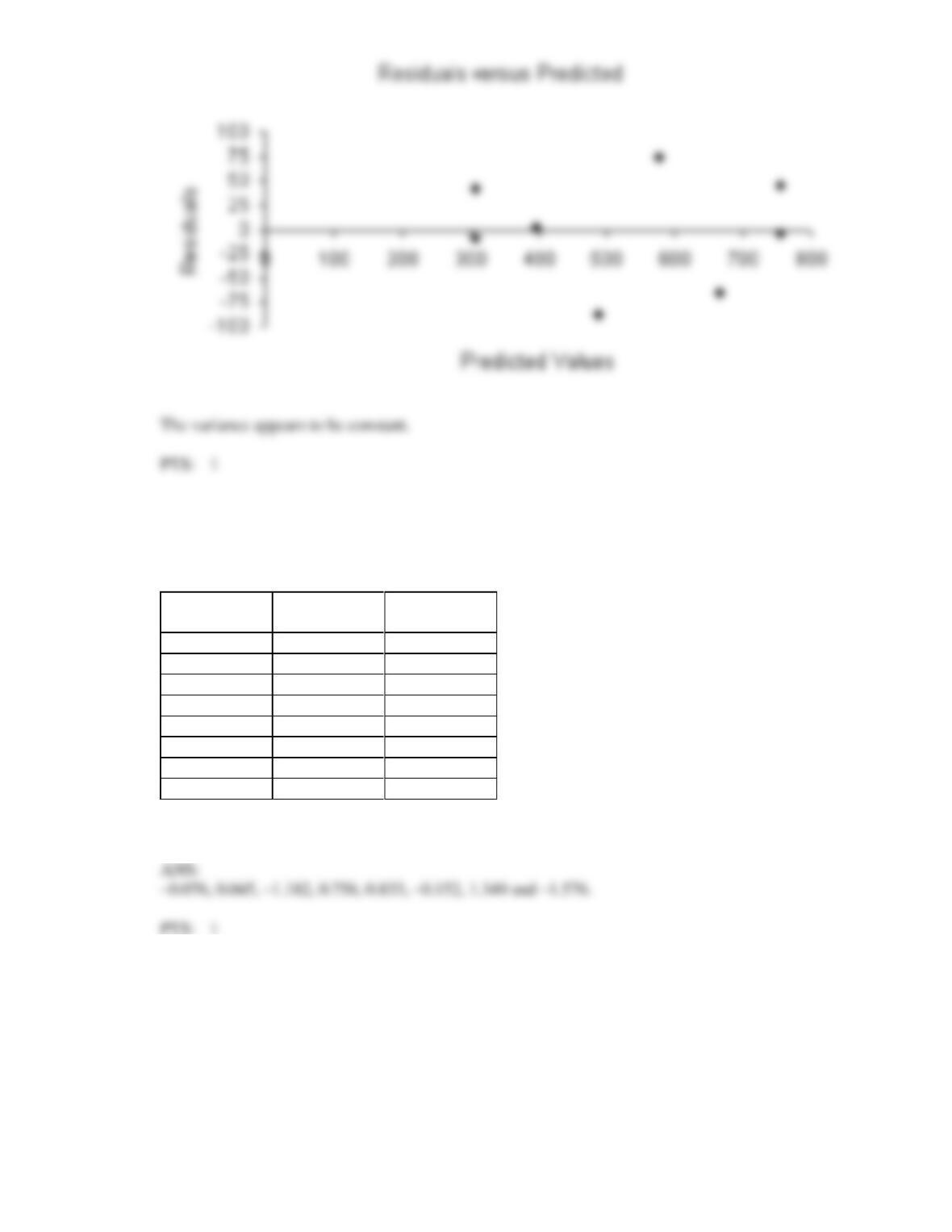
63. Plot the residuals against the predicted values
ö
y
. Does the variance appear to be constant?
ANS:
64. An ardent fan of television game shows has observed that, in general, the more educated the
contestant, the less money he or she wins. To test her belief, she gathers data about the last eight
winners of her favourite game show. She records their winnings in dollars and their years of education.
The results are as follows.
Contestant
Years of
education
Winnings
1
11
750
2
15
400
3
12
600
4
16
350
5
11
800
6
16
300
7
13
650
8
14
400
Compute the standardised residuals.
65. An ardent fan of television game shows has observed that, in general, the more educated the
contestant, the less money he or she wins. To test her belief, she gathers data about the last eight
winners of her favourite game show. She records their winnings in dollars and their years of education.
The results are as follows.

Contestant
Years of
education
Winnings
1
11
750
2
15
400
3
12
600
4
16
350
5
11
800
6
16
300
7
13
650
8
14
400
Identify possible outliers.
66. A financier whose specialty is investing in movie productions has observed that, in general, movies
with ‘big-name’ stars seem to generate more revenue than those movies whose stars are less well
known. To examine his belief, he records the gross revenue and the payment (in $ million) given to the
two highest-paid performers in the movie for 10 recently released movies.
Movie
Cost of two highest-
paid performers ($m)
Gross revenue
($m)
1
5.3
48
2
7.2
65
3
1.3
18
4
1.8
20
5
3.5
31
6
2.6
26
7
8.0
73
8
2.4
23
9
4.5
39
10
6.7
58
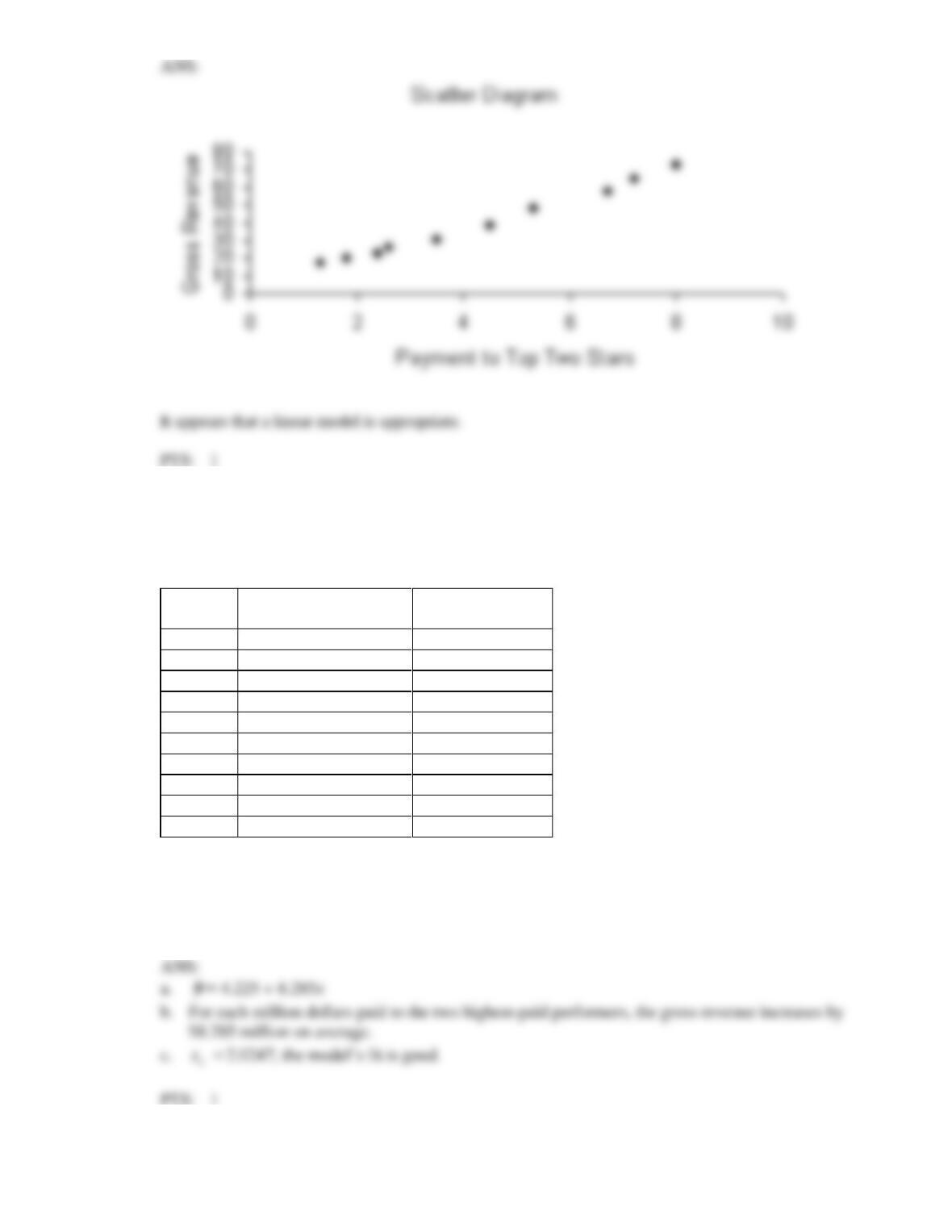
Draw a scatter diagram of the data to determine whether a linear model appears to be appropriate.
67. A financier whose specialty is investing in movie productions has observed that, in general, movies
with ‘big-name’ stars seem to generate more revenue than those movies whose stars are less well
known. To examine his belief, he records the gross revenue and the payment (in $ million) given to the
two highest-paid performers in the movie for 10 recently released movies.
Movie
Cost of two highest-
paid performers ($m)
Gross revenue
($m)
1
5.3
48
2
7.2
65
3
1.3
18
4
1.8
20
5
3.5
31
6
2.6
26
7
8.0
73
8
2.4
23
9
4.5
39
10
6.7
58
a. Determine the least squares regression line.
b. Interpret the value of the slope of the regression line.
c. Determine the standard error of estimate, and describe what this statistic tells you about the
regression line.

68. A financier whose specialty is investing in movie productions has observed that, in general, movies
with ‘big-name’ stars seem to generate more revenue than those movies whose stars are less well
known. To examine his belief, he records the gross revenue and the payment (in $ million) given to the
two highest-paid performers in the movie for 10 recently released movies.
Movie
Cost of two highest-
paid performers ($m)
Gross revenue
($m)
1
5.3
48
2
7.2
65
3
1.3
18
4
1.8
20
5
3.5
31
6
2.6
26
7
8.0
73
8
2.4
23
9
4.5
39
10
6.7
58
Determine the coefficient of determination, and discuss what its value tells you about the two
variables.
69. A financier whose specialty is investing in movie productions has observed that, in general, movies
with ‘big-name’ stars seem to generate more revenue than those movies whose stars are less well
known. To examine his belief, he records the gross revenue and the payment (in $ million) given to the
two highest-paid performers in the movie for 10 recently released movies.
Movie
Cost of two highest-
paid performers ($m)
Gross revenue
($m)
1
5.3
48
2
7.2
65
3
1.3
18
4
1.8
20
5
3.5
31
6
2.6
26
7
8.0
73
8
2.4
23
9
4.5
39
10
6.7
58
Calculate the Pearson correlation coefficient. What sign does it have? Why?

70. A financier whose specialty is investing in movie productions has observed that, in general, movies
with ‘big-name’ stars seem to generate more revenue than those movies whose stars are less well
known. To examine his belief, he records the gross revenue and the payment (in $ million) given to the
two highest-paid performers in the movie for 10 recently released movies.
Movie
Cost of two highest-
paid performers ($m)
Gross revenue
($m)
1
5.3
48
2
7.2
65
3
1.3
18
4
1.8
20
5
3.5
31
6
2.6
26
7
8.0
73
8
2.4
23
9
4.5
39
10
6.7
58
Conduct a test of the population coefficient of correlation to determine at the 5% significance level
whether a linear relationship exists between payment to the two highest-paid performers and gross
revenue.
71. A financier whose specialty is investing in movie productions has observed that, in general, movies
with ‘big-name’ stars seem to generate more revenue than those movies whose stars are less well
known. To examine his belief, he records the gross revenue and the payment (in $ million) given to the
two highest-paid performers in the movie for 10 recently released movies.
Movie
Cost of two highest-
paid performers ($m)
Gross revenue
($m)
1
5.3
48
2
7.2
65
3
1.3
18
4
1.8
20
5
3.5
31
6
2.6
26
7
8.0
73
8
2.4
23
9
4.5
39
10
6.7
58

Conduct a test of the population slope to determine at the 5% significance level whether a linear
relationship exists between payment to the two highest-paid performers and gross revenue.
72. Do the tests provide the same results? Explain.
73. A financier whose specialty is investing in movie productions has observed that, in general, movies
with ‘big-name’ stars seem to generate more revenue than those movies whose stars are less well
known. To examine his belief, he records the gross revenue and the payment (in $ million) given to the
two highest-paid performers in the movie for 10 recently released movies.
Movie
Cost of two highest-
paid performers ($m)
Gross revenue
($m)
1
5.3
48
2
7.2
65
3
1.3
18
4
1.8
20
5
3.5
31
6
2.6
26
7
8.0
73
8
2.4
23
9
4.5
39
10
6.7
58
Assume that the conditions for the tests conducted in the previous two questions are not met. Do the
data allow us to infer at the 5% significance level that payment to the two highest-paid performers and
gross revenue are linearly related?

74. A financier whose specialty is investing in movie productions has observed that, in general, movies
with ‘big-name’ stars seem to generate more revenue than those movies whose stars are less well
known. To examine his belief, he records the gross revenue and the payment (in $ million) given to the
two highest-paid performers in the movie for 10 recently released movies.
Movie
Cost of two highest-
paid performers ($m)
Gross revenue
($m)
1
5.3
48
2
7.2
65
3
1.3
18
4
1.8
20
5
3.5
31
6
2.6
26
7
8.0
73
8
2.4
23
9
4.5
39
10
6.7
58
Predict with 95% confidence the gross revenue of a movie whose top two stars earn $5.0 million.
75. A financier whose specialty is investing in movie productions has observed that, in general, movies
with ‘big-name’ stars seem to generate more revenue than those movies whose stars are less well
known. To examine his belief, he records the gross revenue and the payment (in $ million) given to the
two highest-paid performers in the movie for 10 recently released movies.
Movie
Cost of two highest-
paid performers ($m)
Gross revenue
($m)
1
5.3
48
2
7.2
65
3
1.3
18
4
1.8
20
5
3.5
31
6
2.6
26
7
8.0
73
8
2.4
23
9
4.5
39
10
6.7
58
Predict with 95% confidence the average gross revenue of a movie whose top two stars earn $5.0
million.

76. A financier whose specialty is investing in movie productions has observed that, in general, movies
with ‘big-name’ stars seem to generate more revenue than those movies whose stars are less well
known. To examine his belief, he records the gross revenue and the payment (in $ million) given to the
two highest-paid performers in the movie for 10 recently released movies.
Movie
Cost of two highest-
paid performers ($m)
Gross revenue
($m)
1
5.3
48
2
7.2
65
3
1.3
18
4
1.8
20
5
3.5
31
6
2.6
26
7
8.0
73
8
2.4
23
9
4.5
39
10
6.7
58
Use the regression equation to determine the predicted values of y.
77. A financier whose specialty is investing in movie productions has observed that, in general, movies
with ‘big-name’ stars seem to generate more revenue than those movies whose stars are less well
known. To examine his belief, he records the gross revenue and the payment (in $ million) given to the
two highest-paid performers in the movie for 10 recently released movies.
Movie
Cost of two highest-
paid performers ($m)
Gross revenue
($m)
1
5.3
48
2
7.2
65
3
1.3
18
4
1.8
20
5
3.5
31
6
2.6
26
7
8.0
73
8
2.4
23
9
4.5
39
10
6.7
58
Use the predicted and actual values of y to calculate the residuals.
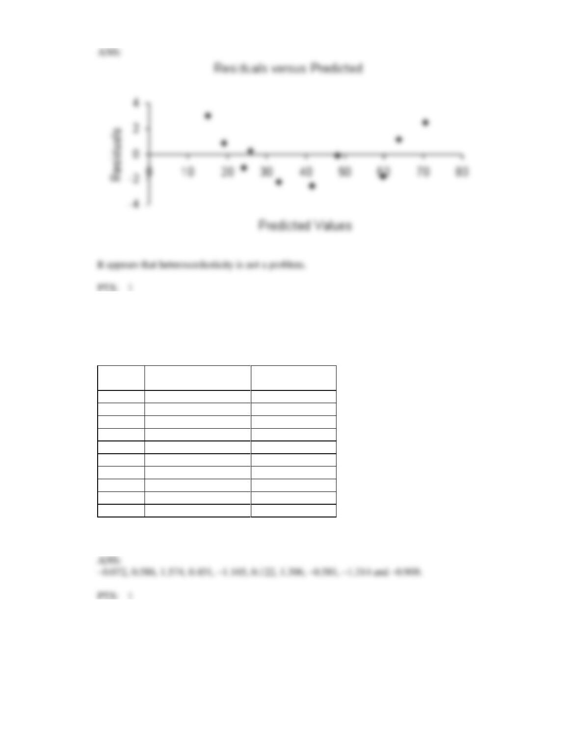
78. Plot the residuals against the predicted values of y. Does the variance appear to be constant?
79. A financier whose specialty is investing in movie productions has observed that, in general, movies
with ‘big-name’ stars seem to generate more revenue than those movies whose stars are less well
known. To examine his belief, he records the gross revenue and the payment (in $ million) given to the
two highest-paid performers in the movie for 10 recently released movies.
Movie
Cost of two highest-
paid performers ($m)
Gross revenue
($m)
1
5.3
48
2
7.2
65
3
1.3
18
4
1.8
20
5
3.5
31
6
2.6
26
7
8.0
73
8
2.4
23
9
4.5
39
10
6.7
58
Compute the standardised residuals.
80. A financier whose specialty is investing in movie productions has observed that, in general, movies
with ‘big-name’ stars seem to generate more revenue than those movies whose stars are less well
known. To examine his belief, he records the gross revenue and the payment (in $ million) given to the
two highest-paid performers in the movie for 10 recently released movies.

Movie
Cost of two highest-
paid performers ($m)
Gross revenue
($m)
1
5.3
48
2
7.2
65
3
1.3
18
4
1.8
20
5
3.5
31
6
2.6
26
7
8.0
73
8
2.4
23
9
4.5
39
10
6.7
58
Identify possible outliers.
81. The editor of a major academic book publisher claims that a large part of the cost of books is the cost
of paper. This implies that larger books will cost more money. As an experiment to analyse the claim,
a university student visits the bookstore and records the number of pages and the selling price of 12
randomly selected books. These data are listed below.
Book
Number of pages
Selling price ($)
1
844
55
2
727
50
3
360
35
4
915
60
5
295
30
6
706
50
7
410
40
8
905
53
9
1058
65
10
865
54
11
677
42
12
912
58
Determine the least squares regression line.
82. The editor of a major academic book publisher claims that a large part of the cost of books is the cost
of paper. This implies that larger books will cost more money. As an experiment to analyse the claim,
a university student visits the bookstore and records the number of pages and the selling price of 12
randomly selected books. These data are listed below.
Book
Number of pages
Selling price ($)
1
844
55
2
727
50
3
360
35
4
915
60
5
295
30
6
706
50
7
410
40
8
905
53
9
1058
65
10
865
54
11
677
42
12
912
58
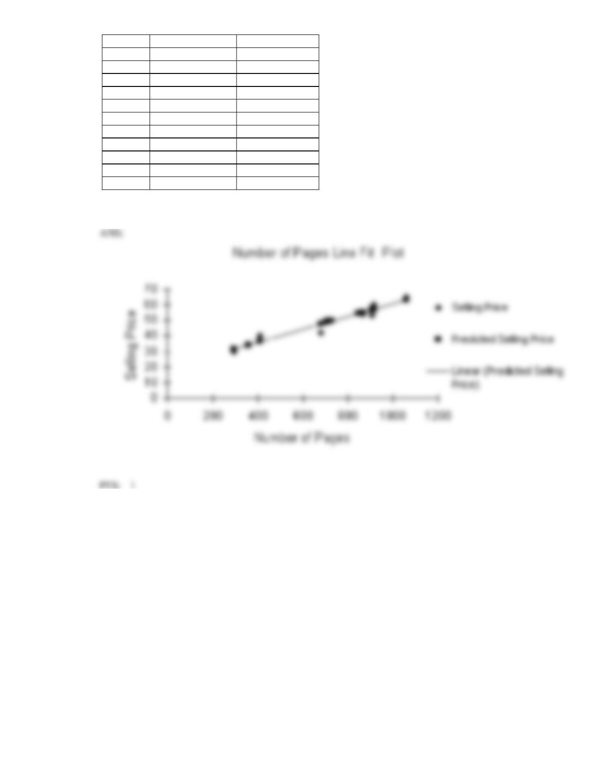
Draw a scatter diagram of the data and plot the least squares regression line on it.
83. The editor of a major academic book publisher claims that a large part of the cost of books is the cost
of paper. This implies that larger books will cost more money. As an experiment to analyse the claim,
a university student visits the bookstore and records the number of pages and the selling price of 12
randomly selected books. These data are listed below.

Book
Number of pages
Selling price ($)
1
844
55
2
727
50
3
360
35
4
915
60
5
295
30
6
706
50
7
410
40
8
905
53
9
1058
65
10
865
54
11
677
42
12
912
58
Interpret the value of the slope of the regression line.
84. The editor of a major academic book publisher claims that a large part of the cost of books is the cost
of paper. This implies that larger books will cost more money. As an experiment to analyse the claim,
a university student visits the bookstore and records the number of pages and the selling price of 12
randomly selected books. These data are listed below.
Book
Number of pages
Selling price ($)
1
844
55
2
727
50
3
360
35
4
915
60
5
295
30
6
706
50
7
410
40
8
905
53
9
1058
65
10
865
54
11
677
42
12
912
58
Determine the coefficient of determination, and discuss what its value tells you.

85. The editor of a major academic book publisher claims that a large part of the cost of books is the cost
of paper. This implies that larger books will cost more money. As an experiment to analyse the claim,
a university student visits the bookstore and records the number of pages and the selling price of 12
randomly selected books. These data are listed below.
Book
Number of pages
Selling price ($)
1
844
55
2
727
50
3
360
35
4
915
60
5
295
30
6
706
50
7
410
40
8
905
53
9
1058
65
10
865
54
11
677
42
12
912
58
Can we infer at the 5% significance level that the editor is correct?
86. The editor of a major academic book publisher claims that a large part of the cost of books is the cost
of paper. This implies that larger books will cost more money. As an experiment to analyse the claim,
a university student visits the bookstore and records the number of pages and the selling price of 12
randomly selected books. These data are listed below.
Book
Number of pages
Selling price ($)
1
844
55
2
727
50
3
360
35
4
915
60
5
295
30
6
706
50
7
410
40
8
905
53
9
1058
65
10
865
54
11
677
42
12
912
58
Estimate with 90% confidence the selling price of a book with 900 pages.

87. The editor of a major academic book publisher claims that a large part of the cost of books is the cost
of paper. This implies that larger books will cost more money. As an experiment to analyse the claim,
a university student visits the bookstore and records the number of pages and the selling price of 12
randomly selected books. These data are listed below.
Book
Number of pages
Selling price ($)
1
844
55
2
727
50
3
360
35
4
915
60
5
295
30
6
706
50
7
410
40
8
905
53
9
1058
65
10
865
54
11
677
42
12
912
58
Estimate with 90% confidence the mean selling price of all books with 900 pages.
88. A statistician investigating the relationship between the amount of precipitation (in inches) and the
number of car accidents gathered data for 10 randomly selected days. The results are presented below.
Day
Precipitation
Number of accidents
1
0.05
5
2
0.12
6
3
0.05
2
4
0.08
4
5
0.10
8
6
0.35
14
7
0.15
7
8
0.30
13
9
0.10
7
10
0.20
10
Find the least squares regression line.

89. A statistician investigating the relationship between the amount of precipitation (in inches) and the
number of car accidents gathered data for 10 randomly selected days. The results are presented below.
Day
Precipitation
Number of accidents
1
0.05
5
2
0.12
6
3
0.05
2
4
0.08
4
5
0.10
8
6
0.35
14
7
0.15
7
8
0.30
13
9
0.10
7
10
0.20
10
Calculate the standard error of estimate, and describe what this statistic tells you about the regression
line.
90. A statistician investigating the relationship between the amount of precipitation (in inches) and the
number of car accidents gathered data for 10 randomly selected days. The results are presented below.
Day
Precipitation
Number of accidents
1
0.05
5
2
0.12
6
3
0.05
2
4
0.08
4
5
0.10
8
6
0.35
14
7
0.15
7
8
0.30
13
9
0.10
7
10
0.20
10
Determine the coefficient of determination and discuss what its value tells you about the two variables.
91. A statistician investigating the relationship between the amount of precipitation (in inches) and the
number of car accidents gathered data for 10 randomly selected days. The results are presented below.


