Unlock document.
This document is partially blurred.
Unlock all pages and 1 million more documents.
Get Access
Calculate the coefficient of determination, and describe what this statistic tells you about the
relationship between the two variables.
10. Consider the following data values of variables x and y.
x
3
5
7
9
11
14
y
7
10
17
20
27
35
Calculate the Pearson coefficient of correlation. What sign does it have? Why?
11. Consider the following data values of variables x and y.
x
3
5
7
9
11
14
y
7
10
17
20
27
35
What does the coefficient of correlation calculated in the previous question tell you about the direction
and strength of the relationship between the two variables?
12. A medical statistician wanted to examine the relationship between the amount of sunshine (x) and
incidence of skin cancer (y). As an experiment he found the number of skin cancers detected per
100 000 of population and the average daily sunshine in eight country towns around NSW. These data
are shown below.
Average daily sunshine (hours)
5
7
6
7
8
6
4
3
Skin cancer per 100 000
7
11
9
12
15
10
7
5
Find the least squares regression line.
13. A medical statistician wanted to examine the relationship between the amount of sunshine (x) and
incidence of skin cancer (y). As an experiment he found the number of skin cancers detected per
100 000 of population and the average daily sunshine in eight country towns around NSW. These data
are shown below.
Average daily sunshine (hours)
5
7
6
7
8
6
4
3
Skin cancer per 100 000
7
11
9
12
15
10
7
5
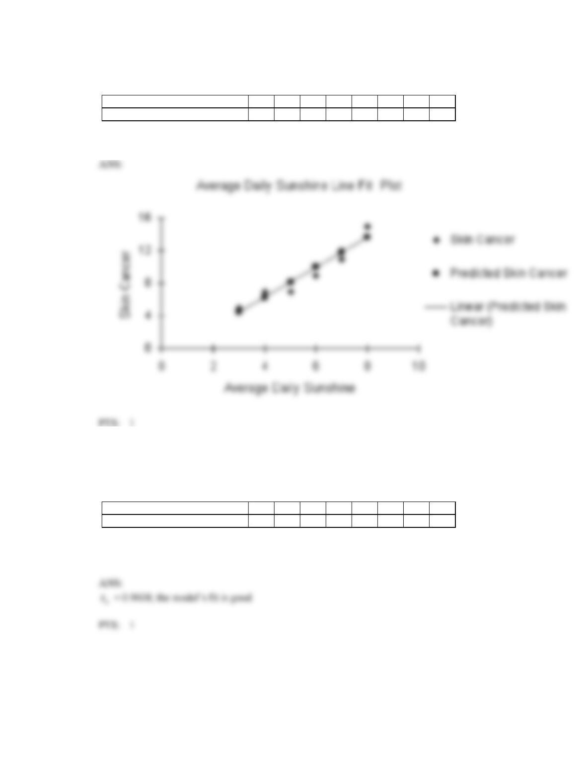
Draw a scatter diagram of the data and plot the least squares regression line on it.
14. A medical statistician wanted to examine the relationship between the amount of sunshine (x) and
incidence of skin cancer (y). As an experiment he found the number of skin cancers detected per
100 000 of population and the average daily sunshine in eight country towns around NSW. These data
are shown below.
Average daily sunshine (hours)
5
7
6
7
8
6
4
3
Skin cancer per 100 000
7
11
9
12
15
10
7
5
Calculate the standard error of estimate, and describe what this statistic tells you about the regression
line.
15. A medical statistician wanted to examine the relationship between the amount of sunshine (x) and
incidence of skin cancer (y). As an experiment he found the number of skin cancers detected per
100 000 of population and the average daily sunshine in eight country towns around NSW. These data
are shown below.
Average daily sunshine (hours)
5
7
6
7
8
6
4
3
Skin cancer per 100 000
7
11
9
12
15
10
7
5
Can we conclude at the 1% significance level that there is a linear relationship between sunshine and
skin cancer?
16. A medical statistician wanted to examine the relationship between the amount of sunshine (x) and
incidence of skin cancer (y). As an experiment he found the number of skin cancers detected per
100 000 of population and the average daily sunshine in eight country towns around NSW. These data
are shown below.
Average daily sunshine (hours)
5
7
6
7
8
6
4
3
Skin cancer per 100 000
7
11
9
12
15
10
7
5
Calculate the coefficient of determination and interpret it.
17. A medical statistician wanted to examine the relationship between the amount of sunshine (x) and
incidence of skin cancer (y). As an experiment he found the number of skin cancers detected per
100 000 of population and the average daily sunshine in eight country towns around NSW. These data
are shown below.
Average daily sunshine (hours)
5
7
6
7
8
6
4
3
Skin cancer per 100 000
7
11
9
12
15
10
7
5
Predict with 95% confidence the incidence of skin cancers per 100 000 in a town with a daily average
of 6.5 hours of sunshine.
18. The manager of a fast food restaurant wishes to determine how sales in a given week are related to the
number of coupons printed in the local newspaper during the week. She records the number of
coupons (x) and sales (y, $) from 10 randomly selected weeks. These data are listed below.
Week
Number of coupons
Sales ($)
1
5
12 560
2
8
16 250
3
6
14 800
4
3
12 100
5
9
17 250
6
10
17 900
7
7
15 800
8
6
15 000
9
2
12 000
10
4
12 800
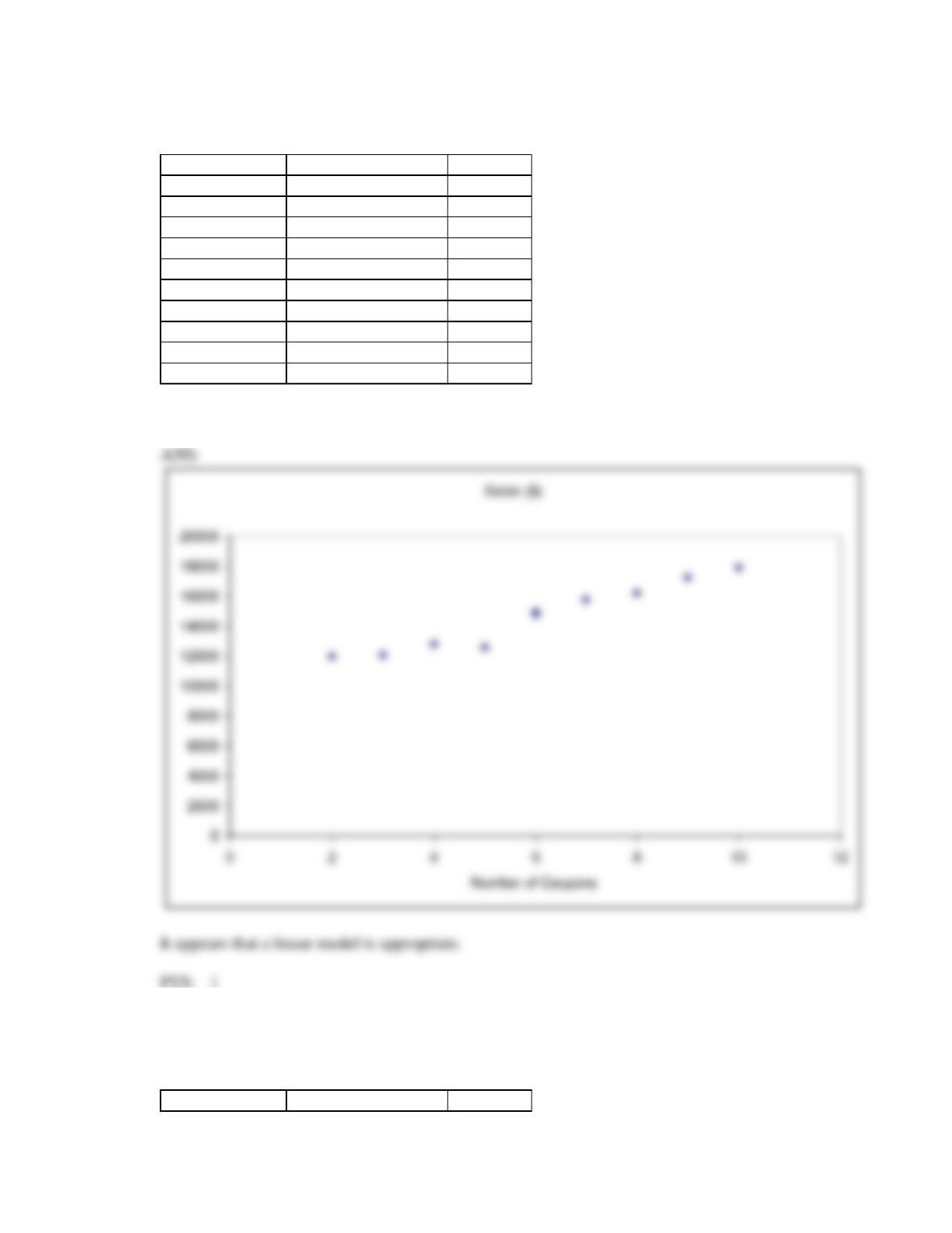
Draw a scatter diagram of the data to determine whether a linear model appears to be appropriate.
19. The manager of a fast food restaurant wishes to determine how sales in a given week are related to the
number of coupons printed in the local newspaper during the week. She records the number of
coupons (x) and sales (y, $) from 10 randomly selected weeks. These data are listed below.
Week
Number of coupons
Sales ($)

1
5
12 560
2
8
16 250
3
6
14 800
4
3
12 100
5
9
17 250
6
10
17 900
7
7
15 800
8
6
15 000
9
2
12 000
10
4
12 800
Determine the least squares regression line.
20. The manager of a fast food restaurant wishes to determine how sales in a given week are related to the
number of coupons printed in the local newspaper during the week. She records the number of
coupons (x) and sales (y, $) from 10 randomly selected weeks. These data are listed below.
Week
Number of coupons
Sales ($)
1
5
12 560
2
8
16 250
3
6
14 800
4
3
12 100
5
9
17 250
6
10
17 900
7
7
15 800
8
6
15 000
9
2
12 000
10
4
12 800
Interpret the value of the slope of the regression line.
21. The manager of a fast food restaurant wishes to determine how sales in a given week are related to the
number of coupons printed in the local newspaper during the week. She records the number of
coupons (x) and sales (y, $) from 10 randomly selected weeks. These data are listed below.
Week
Number of coupons
Sales ($)
1
5
12 560
2
8
16 250
3
6
14 800
4
3
12 100
5
9
17 250
6
10
17 900
7
7
15 800
8
6
15 000
9
2
12 000
10
4
12 800
Determine the standard error of estimate, and describe what this statistic tells you about the regression
line.
22. The manager of a fast food restaurant wishes to determine how sales in a given week are related to the
number of coupons printed in the local newspaper during the week. She records the number of
coupons (x) and sales (y, $) from 10 randomly selected weeks. These data are listed below.
Week
Number of coupons
Sales ($)
1
5
12 560
2
8
16 250
3
6
14 800
4
3
12 100
5
9
17 250
6
10
17 900
7
7
15 800
8
6
15 000
9
2
12 000
10
4
12 800
Determine the coefficient of determination, and discuss what its value tells you about the two
variables.
23. The manager of a fast food restaurant wishes to determine how sales in a given week are related to the
number of coupons printed in the local newspaper during the week. She records the number of
coupons (x) and sales (y, $) from 10 randomly selected weeks. These data are listed below.
Week
Number of coupons
Sales ($)
1
5
12 560
2
8
16 250
3
6
14 800
4
3
12 100
5
9
17 250
6
10
17 900
7
7
15 800
8
6
15 000
9
2
12 000
10
4
12 800
Calculate the Pearson correlation coefficient. What sign does it have? Why?
24. The manager of a fast food restaurant wishes to determine how sales in a given week are related to the
number of coupons printed in the local newspaper during the week. She records the number of
coupons (x) and sales (y, $) from 10 randomly selected weeks. These data are listed below.
Week
Number of coupons
Sales ($)
1
5
12 560
2
8
16 250
3
6
14 800
4
3
12 100
5
9
17 250
6
10
17 900
7
7
15 800
8
6
15 000
9
2
12 000
10
4
12 800
Conduct a test of the population coefficient of correlation to determine at the 5% significance level
whether a linear relationship exists between years of experience and sales.
25. The manager of a fast food restaurant wishes to determine how sales in a given week are related to the
number of coupons printed in the local newspaper during the week. She records the number of
coupons (x) and sales (y, $) from 10 randomly selected weeks. These data are listed below.
Week
Number of coupons
Sales ($)
1
5
12 560
2
8
16 250
3
6
14 800
4
3
12 100
5
9
17 250
6
10
17 900
7
7
15 800
8
6
15 000
9
2
12 000
10
4
12 800
Conduct a test of the population slope to determine at the 5% significance level whether a linear relationship
exists between years of experience and sales.
26. Do the tests in Short Answers 24 and 25 above provide the same results? Explain.
27. Assume that the conditions for the t-tests conducted in Short Answers 24 and 25 above are not met so
that one has to use a non-parametric alternative. Do the data allow us to infer at the 5% significance
level that the number of coupons and weekly sales are linearly related?
28. The manager of a fast food restaurant wishes to determine how sales in a given week are related to the
number of coupons printed in the local newspaper during the week. She records the number of
coupons (x) and sales (y, $) from 10 randomly selected weeks. These data are listed below.
Week
Number of coupons
Sales ($)
1
5
12 560
2
8
16 250
3
6
14 800
4
3
12 100
5
9
17 250
6
10
17 900
7
7
15 800

8
6
15 000
9
2
12 000
10
4
12 800
Predict with 95% confidence the weekly sales for a week when 10 coupons are printed in the local
newspaper.
29. The manager of a fast food restaurant wishes to determine how sales in a given week are related to the
number of coupons printed in the local newspaper during the week. She records the number of
coupons (x) and sales (y, $) from 10 randomly selected weeks. These data are listed below.
Week
Number of coupons
Sales ($)
1
5
12 560
2
8
16 250
3
6
14 800
4
3
12 100
5
9
17 250
6
10
17 900
7
7
15 800
8
6
15 000
9
2
12 000
10
4
12 800
Estimate with 95% confidence the weekly sales for all weeks when 10 coupons are printed in the local
newspaper.
30. The manager of a fast food restaurant wishes to determine how sales in a given week are related to the
number of coupons printed in the local newspaper during the week. She records the number of
coupons (x) and sales (y, $) from 10 randomly selected weeks. These data are listed below.
Week
Number of coupons
Sales ($)
1
5
12 560
2
8
16 250
3
6
14 800
4
3
12 100
5
9
17 250
6
10
17 900
7
7
15 800
8
6
15 000
9
2
12 000
10
4
12 800
Use the regression equation to determine the predicted values of y.
31. The manager of a fast food restaurant wishes to determine how sales in a given week are related to the
number of coupons printed in the local newspaper during the week. She records the number of
coupons (x) and sales (y, $) from 10 randomly selected weeks. These data are listed below.
Week
Number of coupons
Sales ($)
1
5
12 560
2
8
16 250
3
6
14 800
4
3
12 100
5
9
17 250
6
10
17 900
7
7
15 800
8
6
15 000
9
2
12 000
10
4
12 800
Use the predicted and actual values of y to calculate the residuals.
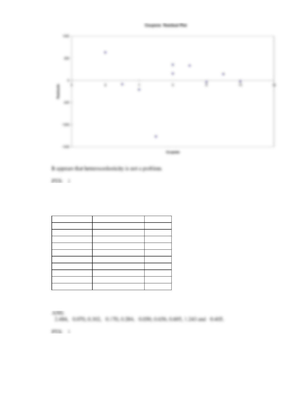
32. Plot the residuals against the predicted values of y. Does the variance appear to be constant?
ANS:
33. The manager of a fast food restaurant wishes to determine how sales in a given week are related to the
number of coupons printed in the local newspaper during the week. She records the number of
coupons (x) and sales (y, $) from 10 randomly selected weeks. These data are listed below.
Week
Number of coupons
Sales ($)
1
5
12 560
2
8
16 250
3
6
14 800
4
3
12 100
5
9
17 250
6
10
17 900
7
7
15 800
8
6
15 000
9
2
12 000
10
4
12 800
Compute the standardised residuals.
34. The manager of a fast food restaurant wishes to determine how sales in a given week are related to the
number of coupons printed in the local newspaper during the week. She records the number of
coupons (x) and sales (y, $) from 10 randomly selected weeks. These data are listed below.
Week
Number of coupons
Sales ($)
1
5
12 560
2
8
16 250
3
6
14 800
4
3
12 100
5
9
17 250
6
10
17 900
7
7
15 800
8
6
15 000
9
2
12 000
10
4
12 800
Identify possible outliers.
35. A professor of economics wants to study the relationship between income y (in $1000s) and education
x (in years). A random sample of eight individuals is taken and the results are shown below.
Education
16
11
15
8
12
10
13
14
Income
58
40
55
35
43
41
52
49
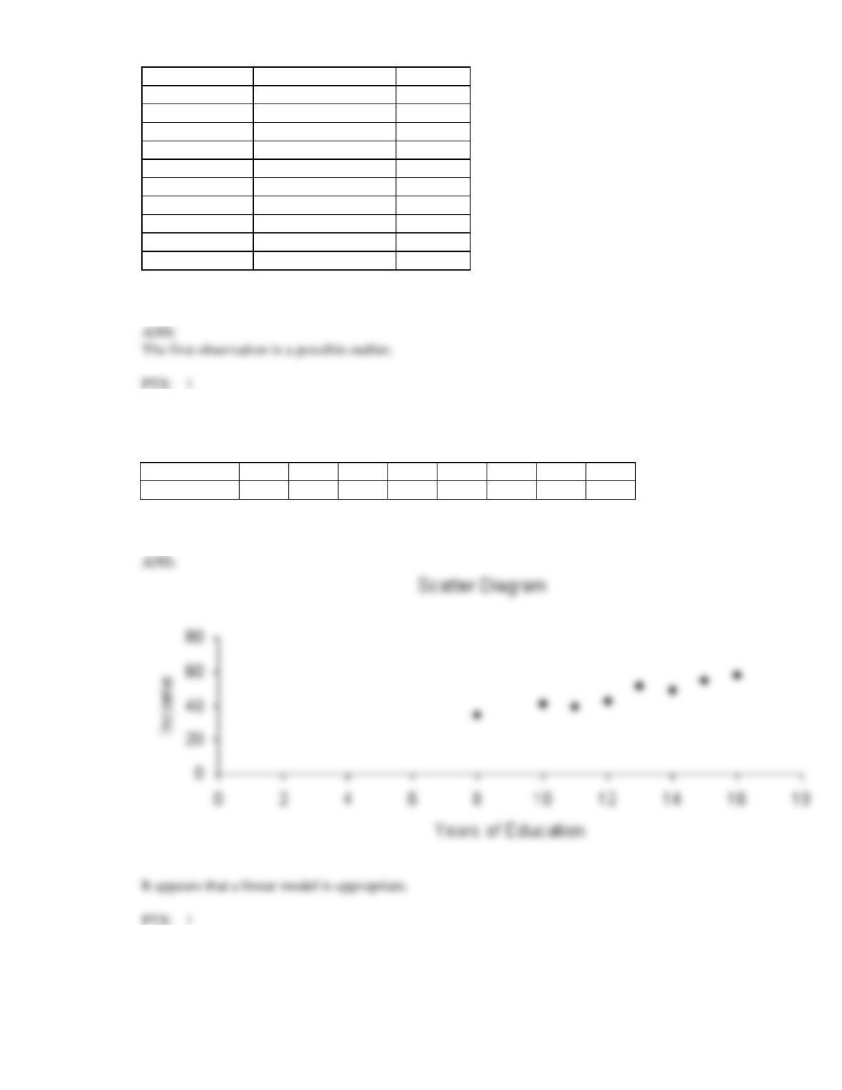
Draw a scatter diagram of the data to determine whether a linear model appears to be appropriate.
36. A professor of economics wants to study the relationship between income y (in $1000s) and education
x (in years). A random sample of eight individuals is taken and the results are shown below.
Education
16
11
15
8
12
10
13
14
Income
58
40
55
35
43
41
52
49
Determine the least squares regression line.
37. A professor of economics wants to study the relationship between income y (in $1000s) and education
x (in years). A random sample of eight individuals is taken and the results are shown below.
Education
16
11
15
8
12
10
13
14
Income
58
40
55
35
43
41
52
49
Interpret the value of the slope of the regression line.
38. A professor of economics wants to study the relationship between income y (in $1000s) and education
x (in years). A random sample of eight individuals is taken and the results are shown below.
Education
16
11
15
8
12
10
13
14
Income
58
40
55
35
43
41
52
49
Determine the standard error of estimate, and describe what this statistic tells you about the regression
line.
39. A professor of economics wants to study the relationship between income y (in $1000s) and education
x (in years). A random sample of eight individuals is taken and the results are shown below.
Education
16
11
15
8
12
10
13
14
Income
58
40
55
35
43
41
52
49
Determine the coefficient of determination, and discuss what its value tells you about the two
variables.
40. A professor of economics wants to study the relationship between income y (in $1000s) and education
x (in years). A random sample of eight individuals is taken and the results are shown below.
Education
16
11
15
8
12
10
13
14
Income
58
40
55
35
43
41
52
49
Calculate the Pearson correlation coefficient. What sign does it have? Why?
41. A professor of economics wants to study the relationship between income y (in $1000s) and education
x (in years). A random sample of eight individuals is taken and the results are shown below.
Education
16
11
15
8
12
10
13
14
Income
58
40
55
35
43
41
52
49
Conduct a test of the population coefficient of correlation to determine at the 5% significance level
whether a linear relationship exists between years of education and income.
42. A professor of economics wants to study the relationship between income y (in $1000s) and education
x (in years). A random sample of eight individuals is taken and the results are shown below.
Education
16
11
15
8
12
10
13
14
Income
58
40
55
35
43
41
52
49
Conduct a test of the population slope to determine at the 5% significance level whether a linear
relationship exists between years of education and income.
43. A professor of economics wants to study the relationship between income y (in $1000s) and education
x (in years). A random sample of eight individuals is taken and the results are shown below.
Education
16
11
15
8
12
10
13
14
Income
58
40
55
35
43
41
52
49
Assume that the conditions for the tests conducted in the previous two questions are not met. Do the
data allow us to infer at the 5% significance level that years of education and income are linearly
related?
44. A professor of economics wants to study the relationship between income y (in $1000s) and education
x (in years). A random sample of eight individuals is taken and the results are shown below.
Education
16
11
15
8
12
10
13
14
Income
58
40
55
35
43
41
52
49
Predict with 95% confidence the income of an individual with 10 years of education.
45. A professor of economics wants to study the relationship between income y (in $1000s) and education
x (in years). A random sample of eight individuals is taken and the results are shown below.
Education
16
11
15
8
12
10
13
14
Income
58
40
55
35
43
41
52
49
Predict with 95% confidence the average income of all individuals with 10 years of education.
46. A professor of economics wants to study the relationship between income y (in $1000s) and education
x (in years). A random sample of eight individuals is taken and the results are shown below.
Education
16
11
15
8
12
10
13
14
Income
58
40
55
35
43
41
52
49
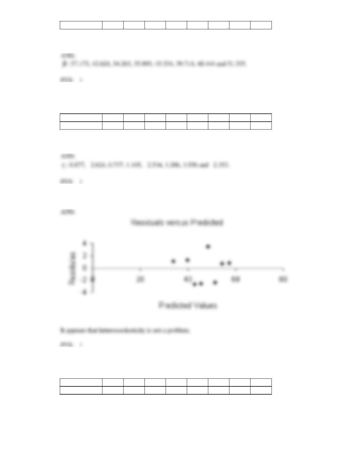
Use the regression equation to determine the predicted values of y.
47. A professor of economics wants to study the relationship between income y (in $1000s) and education
x (in years). A random sample of eight individuals is taken and the results are shown below.
Education
16
11
15
8
12
10
13
14
Income
58
40
55
35
43
41
52
49
Use the predicted and actual values of y to calculate the residuals.
48. Plot the residuals against the predicted values of y. Does the variance appear to be constant?
49. A professor of economics wants to study the relationship between income y (in $1000s) and education
x (in years). A random sample of eight individuals is taken and the results are shown below.
Education
16
11
15
8
12
10
13
14
Income
58
40
55
35
43
41
52
49
Compute the standardised residuals.

50. A professor of economics wants to study the relationship between income y (in $1000s) and education
x (in years). A random sample of eight individuals is taken and the results are shown below.
Education
16
11
15
8
12
10
13
14
Income
58
40
55
35
43
41
52
49
Identify possible outliers.
51. An ardent fan of television game shows has observed that, in general, the more educated the
contestant, the less money he or she wins. To test her belief, she gathers data about the last eight
winners of her favourite game show. She records their winnings in dollars and their years of education.
The results are as follows.
Contestant
Years of
education
Winnings
1
11
750
2
15
400
3
12
600
4
16
350
5
11
800
6
16
300
7
13
650
8
14
400
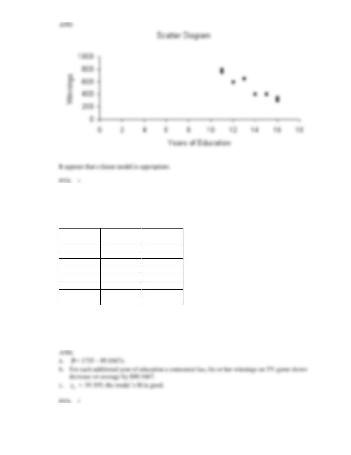
Draw a scatter diagram of the data to determine whether a linear model appears to be appropriate.
52. An ardent fan of television game shows has observed that, in general, the more educated the
contestant, the less money he or she wins. To test her belief, she gathers data about the last eight
winners of her favourite game show. She records their winnings in dollars and their years of
education. The results are as follows.
Contestant
Years of
education
Winnings
1
11
750
2
15
400
3
12
600
4
16
350
5
11
800
6
16
300
7
13
650
8
14
400
a. Determine the least squares regression line.
b. Interpret the value of the slope of the regression line.
c. Determine the standard error of estimate, and describe what this statistic tells you about the
regression line.
53. An ardent fan of television game shows has observed that, in general, the more educated the
contestant, the less money he or she wins. To test her belief, she gathers data about the last eight
winners of her favourite game show. She records their winnings in dollars and their years of education.
The results are as follows.
Contestant
Years of
education
Winnings
1
11
750
2
15
400
3
12
600
4
16
350
5
11
800
6
16
300
7
13
650
8
14
400
Determine the coefficient of determination and discuss what its value tells you about the two variables.
54. An ardent fan of television game shows has observed that, in general, the more educated the
contestant, the less money he or she wins. To test her belief, she gathers data about the last eight
winners of her favourite game show. She records their winnings in dollars and their years of education.
The results are as follows.
Contestant
Years of
education
Winnings
1
11
750
2
15
400
3
12
600
4
16
350
5
11
800
6
16
300
7
13
650
8
14
400
Calculate the Pearson correlation coefficient. What sign does it have? Why?
55. An ardent fan of television game shows has observed that, in general, the more educated the
contestant, the less money he or she wins. To test her belief, she gathers data about the last eight
winners of her favourite game show. She records their winnings in dollars and their years of education.
The results are as follows.
Contestant
Years of
education
Winnings
1
11
750
2
15
400
3
12
600
4
16
350
5
11
800
6
16
300
7
13
650
8
14
400
Conduct a test of the population coefficient of correlation to determine at the 5% significance level
whether a linear relationship exists between TV game show contestants’ years of education and their
winnings.
56. An ardent fan of television game shows has observed that, in general, the more educated the
contestant, the less money he or she wins. To test her belief, she gathers data about the last eight
winners of her favourite game show. She records their winnings in dollars and their years of education.
The results are as follows.
Contestant
Years of
education
Winnings
1
11
750
2
15
400
3
12
600
4
16
350
5
11
800
6
16
300
7
13
650
8
14
400
Conduct a test of the population slope to determine at the 5% significance level whether a linear
relationship exists between TV game show contestants’ years of education and their winnings.


