
Chapter 20—Additional tests for nominal data: Chi-squared tests
MULTIPLE CHOICE
1. Which statistical technique is appropriate when we describe a single population of nominal data with
exactly two categories?
A.
The z-test of a population proportion.
B.
The chi-squared test of a multinomial experiment.
C.
The chi-squared test of a contingency table.
D.
Both A and B.
E.
Both B and C.
2. If we want to conduct a two-tail test of a population proportion, we can employ:
A.
the z-test of a population proportion.
B.
the chi-squared test of a binomial experiment since
22
=z
.
C.
the chi-squared test of a contingency table.
D.
both A and B.
E.
both B and C.
3. Which statistical technique is appropriate when we wish to analyse the relationship between two
nominal variables with two or more categories?
A.
The chi-squared test of a multinomial experiment.
B.
The chi-squared test of a contingency table.
C.
The t-test of the difference between two means.
D.
Both A and B.
E.
Both B and C.
4. If we want to conduct a one-tail test of a population proportion, we can employ:
A.
the z-test of a population proportion.
B.
the chi-squared test of a binomial experiment since
22
=z
.
C.
the chi-squared test of a contingency table.
D.
both A and B.
E.
both B and C.
5. In a goodness-of-fit test, suppose that the value of the test statistic is 20.08 and df = 9. At the 1%
significance level, the null hypothesis is:
A.
rejected and the p–value for the test is smaller than 0.01.
B.
not rejected, and the p-value for the test is greater than 0.01 but smaller than 0.025.
C.
rejected, and the p-value for the test is greater than 0.01 but smaller than 0.025.
D.
not rejected, and the p-value for the test is smaller than 0.01.

6. In a goodness-of-fit test, suppose that a sample showed that the observed frequency
i
f
and expected
frequency
i
e
were equal for each cell i. Then the null hypothesis is:
A.
rejected at
=
0.05 but is not rejected at
=
0.025.
B.
not rejected at
=
0.05 but is rejected at
=
0.025.
C.
rejected at any level
.
D.
not rejected at any
level.
7. The vice-chancellor of a university collected data from students concerning the building of a new
library, and classified the responses into different categories (strongly agree, agree, undecided,
disagree, strongly disagree) and according to whether the student was male or female. To determine
whether the data provide sufficient evidence to indicate that the responses depend upon gender, the
most appropriate test is the:
A.
chi-squared goodness-of-fit test.
B.
chi-squared test of a contingency table (test of independence).
C.
chi-squared test of normality.
D.
chi-squared test for comparing five proportions.
8. The number of degrees of freedom for a contingency table with 6 rows and 4 columns is:
A.
18.
B.
24.
C.
20.
D.
15.
9. A chi-squared test of a contingency table with 4 rows and 4 columns shows that the value of the test
statistic is 22.18. The most accurate statement that can be made about the p-value for this test is that:
A.
the p-value is greater than 0.005 but smaller than 0.01.
B.
the p-value is smaller than 0.01.
C.
the p-value is greater than 0.10.
D.
the p-value is smaller than 0.005.
10. The number of degrees of freedom for a contingency table with 4 rows and 8 columns is:
A.
32.
B.
28.
C.
24.
D.
21.
11. The chi-squared distribution is used:
A.
in a goodness-of-fit test.
B.
in a test of a contingency table.
C.
in making inferences about a single population variance.
D.
All of the above answers are correct.

12. To determine whether a single coin is fair, the coin was tossed 100 times, and heads was observed 55
times. The value of the chi-squared test statistic is:
A.
0.55.
B.
0.50.
C.
1.
D.
55.
13. To determine whether data were drawn from any distribution, we use:
A.
a chi-squared goodness-of-fit test.
B.
a chi-squared test of a contingency table.
C.
a chi-squared test for normality.
D.
None of the above answers is correct.
14. A chi-squared goodness-of-fit test is always conducted as:
A.
a lower-tail test.
B.
an upper-tail test.
C.
a two-tail test.
D.
either A or B.
15. Contingency tables are used in:
A.
testing independence of two samples.
B.
testing dependence in matched pairs.
C.
testing independence of two nominal variables in a population.
D.
describing a single population.
16. The number of degrees of freedom in testing for normality is the:
A.
number of intervals used to test the hypothesis minus 1.
B.
number of parameters estimated minus 1.
C.
number of intervals used to test the hypothesis minus the number of parameters estimated
minus 1.
D.
number of intervals used to test the hypothesis minus the number of parameters estimated
minus 2.
17. If the expected frequency
i
e
for any cell i is less than 5, we:
A.
must choose another sample of five or more observations.
B.
should use the normal distribution instead of the chi-squared distribution.
C.
should combine the cells such that each observed frequency
i
f
is 5 or more.
D.
increase the number of degrees of freedom for the test by 5.

18. If each element in a population is classified into one and only one of several categories, the population
is a:
A.
normal population.
B.
multinomial population.
C.
chi-squared population.
D.
binomial population.
19. To determine the critical values in the chi-squared distribution table, the process requires which of the
following information?
A.
Degrees of freedom.
B.
Probability of Type I error.
C.
Probability of Type II error.
D.
Both A and B.
20. Of the values for a chi-squared test statistic listed below, which one is likely to lead to rejection of the
null hypothesis in a goodness-of-fit test?
A.
0.
B.
1.
C.
2.
D.
40.
21. The number of degrees of freedom in a test of a contingency table with 7 rows and 5 columns is:
A.
24.
B.
35.
C.
30.
D.
28.
22. Which statistical technique is appropriate when we describe a single population of nominal data with
two or more categories?
A.
The z-test of the difference between two proportions.
B.
The chi-squared test of a multinomial experiment.
C.
The chi-squared test of a contingency table.
D.
Both A and B.
E.
Both B and C.
23. The sampling distribution of the test statistic for a goodness-of-fit test with k categories is the:
A.
Student t-distribution with k – 1 degrees of freedom.
B.
normal distribution.
C.
chi-squared distribution with k – 1 degrees of freedom.
D.
approximately chi-squared distribution with k – 1 degrees of freedom.

24. The chi-squared test of a contingency table is based upon:
A.
two nominal variables.
B.
two numerical variables.
C.
three or more nominal variables.
D.
three or more numerical variables.
25. Which of the following statements is not correct?
A.
The chi-squared distribution is symmetrical.
B.
The chi-squared distribution is skewed to the right.
C.
All values of the chi-squared distribution are positive.
D.
The critical region for a goodness-of-fit test with k categories is
2
1,
2
−
k
.
26. Which statistical technique is appropriate when we compare two populations of nominal data with
exactly two categories?
A.
The z-test of a population proportion.
B.
The z-test of the difference between two proportions.
C.
The chi-squared test of a contingency table.
D.
Both A and B.
E.
Both B and C.
27. Which of the following statements is not correct?
A.
The chi-squared test of independence is a one-sample test.
B.
Both variables in the chi-squared test of independence are nominal variables.
C.
The chi-squared goodness-of-fit test involves two categorical variables.
D.
The chi-squared distribution is skewed to the right.
28. A left-tailed area in the chi-squared distribution equals 0.975. For df = 11, the table value equals:
A.
20.4831.
B.
19.6751.
C.
3.81575.
D.
21.9200.
29. Which of the following statements is true for the chi-squared tests?
A.
Testing for equal proportions is identical to testing for goodness-of-fit.
B.
The number of degrees of freedom in a test of a contingency table with r rows and c
columns is (r – 1)(c – 1).
C.
The number of degrees of freedom in a goodness-of-fit test with k categories is k – 1.
D.
All of the above statements are true.

30. The degrees of freedom in a chi-squared test for normality, where the number of standardised intervals
is 13 and there are 2 population parameters to be estimated from the data, is equal to:
A.
13.
B.
10.
C.
11.
D.
2.
31. A chi-squared test for independence with 6 degrees of freedom results in a test statistic
58.13
2=
.
Using the
2
tables, the most accurate statement that can be made about the p-value for this test is that:
A.
p-value > 0.10.
B.
p-value > 0.05.
C.
0.05 < p-value < 0.10.
D.
0.025 < p-value < 0.05.
32. In a goodness-of-fit test, the null hypothesis states that the data came from a normally distributed
population. The researcher estimated the population mean and population standard deviation from a
sample of 500 observations. In addition, the researcher used 6 standardised intervals to test for
normality. Using a 5% level of significance, the critical value for this test is:
A.
11.1433.
B.
9.3484.
C.
7.8147.
D.
9.4877.
33. In a chi-squared test of a contingency table, the value of the test statistic was
678.12
2=
, the
significance level was
= 0.05 and the degrees of freedom was 6. Thus:
A.
we fail to reject the null hypothesis at
= 0.05.
B.
we reject the null hypothesis at
= 0.05.
C.
we don’t have enough evidence to accept or reject the null hypothesis at
= 0.05.
D.
we should increase the level of significance in order to reject the null hypothesis.
34. Which statistical technique is appropriate when we compare two or more populations of nominal data
with two or more categories?
A.
The z-test of the difference between two proportions.
B.
The chi-squared test of a multinomial experiment.
C.
The chi-squared test of a contingency table.
D.
Both A and B.
E.
Both B and C.

35. Which of the following tests does not use the chi-squared distribution?
A.
Test of a contingency table.
B.
Goodness-of-fit test.
C.
Difference between two population means test.
D.
All of the above tests use the chi-squared distribution.
36. Which statistical technique is appropriate when we compare two populations of nominal data with two
or more categories?
A.
The z-test of the difference between two proportions.
B.
The chi-squared test of a multinomial experiment.
C.
The chi-squared test of a contingency table.
D.
Both A and B.
E.
Both B and C.
37. Which of the following is not a characteristic of a multinomial experiment?
A.
The experiment consists of a fixed number, n, of trials.
B.
The outcome of each trial can be classified into one of two categories called success and
failure.
C.
The probability
i
p
that the outcome will fall into cell i remain constant for each trial.
D.
Each trial of the experiment is independent of the other trials.
38. In a chi-squared goodness-of-fit test, if the expected frequencies
i
e
and the observed frequencies
i
f
were quite different, we would conclude that:
A.
the null hypothesis is false, and we would reject it.
B.
the null hypothesis is true, and we would not reject it.
C.
the alternative hypothesis is false, and we would reject it.
D.
the chi-squared distribution is invalid, and we would use the t-distribution instead.
39. In chi-squared tests, the conventional and conservative rule – known as the rule of five – is to require
that the:
A.
expected frequency for each cell be at least 5.
B.
number of degrees of freedom for the test be at least 5.
C.
each expected and observed frequency be at least 5.
D.
difference between the observed and expected frequency for each cell be at least 5.
40. Consider a multinomial experiment with 100 trials, and the outcome of each trial can be classified into
one of 4 categories. The number of degrees of freedom associated with the chi-squared goodness-of-fit
test is:
A.
99.
B.
104.
C.
96.
D.
3.

TRUE/FALSE
1. The null hypothesis states that the sample data came from a normally distributed population. The
researcher calculates the sample mean and the sample standard deviation from the data. The data
arrangement consisted of seven categories. Using a 0.05 significance level, the appropriate critical
value for this chi-squared test for normality is 11.0705.
2. A test for independence is applied to a contingency table with 2 rows and 7 columns for two nominal
variables. The number of degrees of freedom for this chi-squared test must be 6.
3. A chi-squared test for independence with 6 degrees of freedom results in a test statistic of 13.25. Using
the chi-squared table, the most accurate statement that can be made about the p-value for this test is
that 0.025 < p-value < 0.05.
4. Whenever the expected frequency of a cell is less than 5, one remedy for this condition is to increase
the significance level.
5. In testing a population mean or constructing a confidence interval for the population mean, an essential
assumption is that expected frequencies are at least 5.
6. A right-tailed area in the chi-squared distribution equals 0.01. For 4 degrees of freedom, the table
value equals 13.2767.
7. Whenever the expected frequency of a cell is less than 5, one remedy for this condition is to increase
the size of the sample.
8. A left-tailed area in the chi-squared distribution equals 0.10. For 5 degrees of freedom, the table value
equals 9.23635.
9. For a chi-squared distributed random variable with 10 degrees of freedom and a level of significance
of 0.025, the chi-squared value from the table is 20.4831. The computed value of the test statistic is
16.857. This will lead us to reject the null hypothesis.

10. A test for independence is applied to a contingency table with 4 rows and 4 columns for two nominal
variables. The number of degrees of freedom for this test will be 9.
11. A chi-squared test for independence with 10 degrees of freedom results in a test statistic of 17.894.
Using the chi-squared table, the most accurate statement that can be made about the p-value for this
test is that 0.05 < p–value < 0.10.
12. Whenever the expected frequency of a cell is less than 5, one possible remedy for this condition is to
combine it with one or more other cells.
13. The middle 0.95 portion of the chi-squared distribution with 9 degrees of freedom has table values of
3.32511 and 16.9190, respectively.
14. In applying the chi-squared goodness-of-fit test, the rule of thumb for all expected frequencies is that
each expected frequency equals or exceeds 5.
15. In a chi-squared test of independence, the value of the test statistic was
2
=
15.652, and the critical
value at
0.025
=
was 11.1433. Thus we must reject the null hypothesis at
0.025
=
.
16. The chi-squared test of independence is based upon three or more numerical variables.
17. In a goodness-of-fit test, the null hypothesis states that the data came from a normally distributed
population. The researcher estimated the population mean and population standard deviation from a
sample of 100 observations. In addition, the researcher used 6 standardised intervals to test for
normality. Using a 2.5% level of significance, the critical value for this test is 9.3484.
18. A chi-squared goodness-of-fit test can be conducted either as a two-tail test or as a one-tail test.
19. A left-tailed area in the chi-squared distribution equals 0.90. For 10 degrees of freedom, the table value
equals 15.9871.

20. For a chi-squared distributed random variable with 12 degrees of freedom and a level of significance
of 0.05, the chi-squared value from the table is 21.0261. The computed value of the test statistics is
25.1687. This will lead us to reject the null hypothesis.
21. In a goodness-of-fit test, the null hypothesis states that the data came from a normally distributed
population. The researcher estimated the population mean and population standard deviation from a
sample of 200 observations. In addition, the researcher used 5 standardised intervals to test for
normality. Using a 10% level of significance, the critical value for this test is 4.60517.
22. In chi-squared tests, the conventional and conservative rule – known as the rule of five – is to require
that difference between the observed and expected frequency for each cell be at least 5.
23. Whenever the expected frequency of a cell is less than 5, one remedy for this condition is to decrease
the significance level.
24. The area to the right of a chi-squared value is 0.01. For 8 degrees of freedom, the table value is
20.0902.
25. A multinomial experiment, where the outcome of each trial can be classified into one of two
categories, is identical to the binomial experiment.
26. The chi-squared goodness-of-fit test is usually used as a test of multinomial parameters, but it can also
be used to determine whether data were drawn from any distribution.
27. The chi-squared test of a contingency table is used to determine if there is enough evidence to infer
that two nominal variables are related, and to infer that differences exist among two or more
populations of nominal variables.
28. The number of degrees of freedom for a contingency table with r rows and c columns is (r − 1)(c − 1),
provided that both r and c are greater than or equal to 5.
29. When the problem objective is to describe a population of nominal data with exactly two categories,
we can employ either the z-test of population proportion p, or the chi-squared goodness-of-fit test.

30. If we want to test for differences between two populations of nominal data with exactly two categories,
we can employ either the z-test of
1 2
p p−
, or the chi-squared test of a contingency table. (Squaring
the value of the z–statistic yields the value of the
2
-statistic.)
31. If we want to perform a two-tail test for differences between two populations of nominal data with
exactly two categories, we can employ either the z-test of
1 2
p p−
, or the chi-squared test of a
contingency table. (Squaring the value of the z-statistic yields the value of the
2
-statistic.)
32. If we want to perform a one-tail test for differences between two populations of nominal data with
exactly two categories, we must employ the z-test of
1 2
p p−
.
33. The number of degrees of freedom associated with the chi-squared test for normality is the number of
intervals used minus the number of parameters estimated from the data.
34. Like that of the Student t-distribution, the shape of the chi-squared distribution depends on its number
of degrees of freedom.
SHORT ANSWER
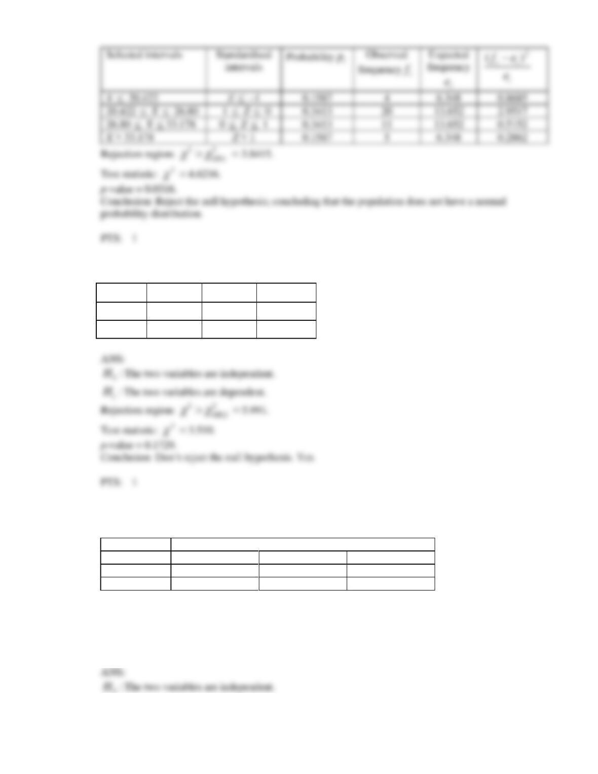
1. The following data are believed to have come from a normal probability distribution.
26
21
25
20
21
29
26
23
22
24
24
30
23
32
26
24
32
16
36
26
21
31
26
23
32
35
40
30
14
26
46
27
33
25
27
21
26
18
29
36
The mean of this sample equals 26.80, and the standard deviation equals 6.378. Use the goodness-of-
fit test at the 5% significance level to test this claim.
2. Conduct a test to determine whether the two classifications A and B are independent, using the data in
the accompanying table and
0.05
=
.
1
B
2
B
3
B
1
A
15
25
30
2
A
25
20
25
The personnel manager of a consumer product company asked a random sample of employees how
they felt about the work they were doing. The following table gives a breakdown of their responses by
gender.
Response
Gender
Very interesting
Fairly interesting
Not interesting
Male
70
41
9
Female
35
34
11
Use this information to answer the following question(s).
3. Do the data provide sufficient evidence to conclude that the level of job satisfaction is related to
gender? Use
=
0.10.
20.422
26.80
4. An Australian firm has been accused of engaging in prejudicial hiring practices. According to the most
recent census, the percentages of whites, Asians and Aborigines in a certain community are 72%, 10%
and 18%, respectively. A random sample of 200 employees of the firm revealed that 165 were white,
14 were Asian, and 21 were Aboriginal. Do the data provide sufficient evidence to conclude at the 5%
level of significance that the firm has been engaged in prejudicial hiring practices?
5. Five brands of orange juice are displayed side by side in several supermarkets in a large city. It was
noted that in one day, 180 customers purchased orange juice. Of these, 30 picked Brand A, 40 picked
Brand B, 25 picked Brand C, 35 picked Brand D, and 50 picked brand E. In this city, can you conclude
at the 5% significance level that there is a preferred brand of orange juice?
6. A sport preference poll showed the following data for men and women:
Favourite Sport
Gender
Rugby
Basketball
Football
Golf
Tennis
Male
24
17
30
18
22
Female
21
20
22
12
28
Using the 5% level of significance, test to determine whether sport preferences depend on gender.

7. Last year, Brand A microwaves had 45% of the market, Brand B had 35% and Brand C had 20%. This
year the makers of Brand C launched a heavy advertising campaign. A random sample of appliance
stores shows that of 10 000 microwaves sold, 4350 were Brand A, 3450 were Brand B, and 2200 were
Brand C. Has the market changed? Test at
=
0.01.
8. A study of educational levels of 500 voters and their political party affiliations in a particular state in
the US showed the following results.
Party Affiliation
Educational level
Democrat
Republican
Independent
Didn’t complete High School
40
20
80
High School Diploma
70
30
60
Has College Degree
90
50
60
Using the 1% level of significance, test to see if party affiliation is independent of the educational level
of the voters.