
A Roadmap for Analyzing Data 18-1
CHAPTER 18: A ROADMAP FOR ANALYZING DATA
1. The probability that a particular brand of smoke alarm will function properly and sound an alarm
in the presence of smoke is 0.8. You have 5 such alarms in your home and they operate
independently. Which of the following distributions would you use to determine the probability
that all of them will function properly in case of a fire?
a) Binomial distribution.
b) Poisson distribution.
c) Normal distribution.
d) Hypergeometric distribution.
2. A certain type of new business succeeds 60% of the time. Suppose that 3 such businesses open
(where they do not compete with each other, so it is reasonable to believe that their relative
successes would be independent). Which of the following distributions would you use to
determine the probability that all of them will fail?
a) Binomial distribution.
b) Poisson distribution.
c) Normal distribution.
d) Hypergeometric distribution.
3. Suppose that past history shows that 60% of college students prefer Coca-Cola. A sample of 10
students is to be selected. Which of the following distributions would you use to figure out the
probability that at least half of them will prefer Coca-Cola?
a) Binomial distribution.
b) Poisson distribution.
c) Normal distribution.
d) Hypergeometric distribution.

18-2 A Roadmap for Analyzing Data
4. Suppose the probability of a power outage at a nuclear power plant on a single day is the same
every day of the year. Also the probability of having a power outage on a single day does not
increase or decrease the probability of a power outage on another day. Which of the following
distributions would you use to determine the probability that a power outage will occur next
Monday?
a) Binomial distribution.
b) Poisson distribution.
c) Normal distribution.
d) Hypergeometric distribution.
5. The probability of receiving a 911 call on a university campus is the same every day. The
probability of having received a 911 call on a single day does not change the probability of
receiving a 911 call on any other day. Which of the following distributions would you use to
determine the probability that a 911 call will be received next day?
a) Binomial distribution.
b) Poisson distribution.
c) Normal distribution.
d) Hypergeometric distribution.
6. An Undergraduate Study Committee of 6 members at a major university is to be formed from a
pool of faculty of 18 men and 6 women. Which of the following distributions would you use to
determine the probability that half of the members will be women?
a) Hypergeometric distribution.
b) Poisson distribution.
c) Uniform distribution.
d) Binomial distribution.
ANSWER:

A Roadmap for Analyzing Data 18-3
7. A debate team of 4 members for a high school will be chosen randomly from a potential group
of 15 students. Ten of the 15 students have no prior competition experience while the others
have some degree of experience. Which of the following distributions would you use to
determine the probability that none of the members chosen for the team have any competition
experience?
a) Hypergeometric distribution.
b) Poisson distribution.
c) Uniform distribution.
d) Binomial distribution.
8. It was believed that the probability of a small business that declared bankruptcy per month was
the same in any month. Also the number of small businesses that declared bankruptcy was the
same every month. Which of the following distributions would you use to determine the
probability that more than 3 bankruptcies will occur next month?
a) Hypergeometric distribution.
b) Poisson distribution.
c) Uniform distribution.
d) Binomial distribution.
9. From an inventory of 48 new cars being shipped to local dealerships, corporate reports indicate
that 12 have defective radios installed. Which of the following distributions would you use to
determine the probability that out of the 8 new cars it just received that, when each is tested, no
more than 2 of the cars have defective radios?
a) Hypergeometric distribution.
b) Poisson distribution.
c) Uniform distribution.
d) Binomial distribution.

18-4 A Roadmap for Analyzing Data
10. The quality control manager of a candy plant is inspecting a batch of chocolate chip bags. When
the production process is in control, the average number of blue chocolate chips per bag is 6.0.
Suppose that the probability of a blue chocolate chip in a bag is constant across bags and the
number of blue chocolate chips in one bag is independent of the number in any other bag. Which
of the following distributions would you use to figure out the probability that any particular bag
being inspected has 4.0 blue chocolate chips?
a) Hypergeometric distribution.
b) Poisson distribution.
c) Uniform distribution.
d) Binomial distribution.
11. The probability that a particular brand of smoke alarm will malfunction in the presence of smoke
is 0.002. A batch of 100,000 such alarms was produced by independent production lines. Which
of the following distributions would you use to figure out the probability that at most 5,000 of
them will malfunction in case of a fire?
a) Hypergeometric distribution.
b) Poisson distribution.
c) Binomial distribution.
d) Uniform distribution.
12. The Tampa International Airport (TIA) has been criticized for the waiting times associated with
departing flights. While the critics acknowledge that many flights have little or no waiting times,
their complaints deal more specifically with the longer waits attributed to some flights. The
critics are interested in showing, mathematically, exactly what the problems are. Which type of
distribution would best model the waiting times of the departing flights at TIA?
a) Uniform distribution
b) Binomial distribution
c) Normal distribution
d) Exponential distribution

A Roadmap for Analyzing Data 18-5
13. It was believed that the probability of being hit by lightning is the same during the course of a
thunderstorm. Which of the following distributions would you use to determine the probability
of being hit by a lightning during the first half of a thunderstorm?
a) Normal distribution.
b) Poisson distribution.
c) Uniform distribution.
d) Exponential distribution.
14. Suppose the probability of producing a defective light bulb from a production line is the same
over an interval of 90 minutes. Which of the following distributions would you use to determine
the probability that a defective light bulb will be produced in a 15 minutes interval?
a) Normal distribution.
b) Poisson distribution.
c) Uniform distribution.
d) Exponential distribution.
15. Suppose the probability of a car accident taking place anywhere on a stretch of a 20 miles
highway is the same. Which of the following distributions would you use to determine the
probability that a car accident will occur somewhere between the 5-mile and 15-mile posts of the
highway?
a) Normal distribution.
b) Poisson distribution.
c) Uniform distribution.
d) Exponential distribution.

18-6 A Roadmap for Analyzing Data
16. Suppose the probability of finding a defective spot in an area on a piece of glass is the ratio of
that area to the total area of the glass and the probability is the same across the whole glass.
Which of the following distributions would you use to determine the probability of finding a
defective spot in a randomly selected one square inch area on a piece of 10 feet by 10 feet glass?
a) Normal distribution.
b) Poisson distribution.
c) Uniform distribution.
d) Exponential distribution.
17. Suppose students arrive at an advising office at a rate of 30 per hour. Which of the following
distributions would you use to determine the probability that the next two students will arrive 30
minutes apart?
a) Normal distribution.
b) Poisson distribution.
c) Uniform distribution.
d) Exponential distribution.
18. Suppose the light bulbs in a factory burn out at a rate of 50 bulbs per month. Which of the
following distributions would you use to determine the probability that the next two light bulbs
will burn out 2 days apart?
a) Hypergeometric distribution.
b) Poisson distribution.
c) Uniform distribution.
d) Exponential distribution.

A Roadmap for Analyzing Data 18-7
19. The amount of juice that can be squeezed from a randomly selected orange out a box of oranges
with approximately the same size can most likely be modeled by which of the following
distributions?
a) Uniform distribution.
b) Poisson distribution.
c) Normal distribution.
d) Exponential distribution.
20. The weight of a randomly selected cookie from a production line can most likely be modeled by
which of the following distributions?
a) Uniform distribution.
b) Poisson distribution.
c) Normal distribution.
d) Exponential distribution.
21. A quality control manager at a plant that produces o-rings is concerned about whether the
diameter of the o-rings that are produced is conformable to the specification. She has calculated
that the average diameter of the o-rings is 4.2 centimeters. She also knows that approximately
95% of the o-rings have diameters fall between 3.2 and 5.2 centimeters and almost all of the o–
rings have diameters between 2.7 and 5.7 centimeters. When modeling the diameters of the o–
rings, which distribution should the scientists use?
a) Uniform distribution
b) Binomial distribution
c) Normal distribution
d) Exponential distribution

18-8 A Roadmap for Analyzing Data
22. A wheel spinning game is played with a special wheel with 24 equal segments that determine the
dollar values of a single spin. Which of the following distributions can best be used to compute
the probability of winning a specific dollar value in a single spin?
a) Uniform distribution
b) Binomial distribution
c) Normal distribution
d) Exponential distribution
23. Suppose that past history shows that 6% of college students prefer Brand A Cola. A sample of
10,000 students is to be selected. Which of the following distributions would you use to
compute the probability that at least half of them will prefer Brand A cola?
a) Hypergeometric distribution.
b) Poisson distribution.
c) Binomial distribution.
d) Uniform distribution.
24. True or False: An insurance company evaluates many variables about a person before deciding
on an appropriate rate for automobile insurance. A representative from a local insurance agency
selected a random sample of 100 insured drivers and recorded, X, the amount of claims each
made in the last 3 years. A Pareto chart can be used to present this information.
25. True or False: At a meeting of information systems officers for regional offices of a national
company, a survey was taken to determine the number of employees the officers supervise in the
operation of their departments, where X is the number of employees overseen by each
information systems officer. A stem-and-leaf display can be used to present this information.

A Roadmap for Analyzing Data 18-9
26. True or False: Every spring semester, the School of Business coordinates a luncheon for
graduating seniors, their families, and friends with local business leaders . Corporate sponsorship
pays for the lunches of each of the seniors, but students have to purchase tickets to cover the cost
of lunches served to guests they bring with them. Data on the number of guests each graduating
senior invited to the luncheon and the number of graduating seniors in each category were
collected. A histogram can be used to present this information.
27. A professor of economics at a small Texas university wanted to determine what year in school
students were taking his tough economics course. Data were collected on the class status
(“freshman”, “sophomore”, “junior” or “senior”) of 50 students enrolled in one of his economics
course. A side-by-side bar chart can be used to present this information.
28. A survey was conducted to determine how people rated the quality of programming available on
television. Respondents were asked to rate the overall quality from 0 (no quality at all) to 100
(extremely good quality). An cumulative percentage polygon (ogive) can be used to present this
information.
29. A sample of 200 students at a Big-Ten university was taken after the midterm to ask whether they
went bar hopping the weekend before the midterm or spent the weekend studying, and whether
they did well or poorly on the midterm. You can use a contingency table to present this
information.
30. The opinions (classified as “for”, “neutral” or “against”) of a sample of 200 people broken down
by gender about the latest congressional plan to eliminate anti-trust exemptions for professional
baseball. You can present this information using a scatter plot.

18-10 A Roadmap for Analyzing Data
31. Data were collected on the amount of detergent used in gallons in a month by 25 drive-through
car wash operations in Phoenix. You can use a time-series plot to pressing this information.
32. Data on the amount of time spent studying and the exam score of 150 students at a high school
were collected. You want to know if a student’s exam score is linearly related to the amount of
time spent on studying. Which of the following would you compute?
a) Arithmetic mean.
b) Median.
c) Coefficient of variation.
d) Coefficient of correlation
33. Data on the amount of time spent studying for a particular exam at a high school were collected
for 150 students. You want to know half of the students spent at least how much time studying
for that exam. Which of the following would you compute?
a) Arithmetic mean.
b) Median.
c) Coefficient of variation.
d) Coefficient of correlation.
34. Data on the amount of money made in a year by 1000 families in a small town were collected.
You want to know the difference in the amount of money made in that year by the middle 50% of
the 1,000 families. Which of the following would you compute?
a) Arithmetic mean.
b) Median.
c) Interquartile Range.
d) Coefficient of correlation.

A Roadmap for Analyzing Data 18-11
35. Every spring semester, the School of Business coordinates with local business leaders a luncheon
for graduating seniors, their families, and friends. Corporate sponsorship pays for the lunches of
each of the seniors, but students have to purchase tickets to cover the cost of lunches served to
guests they bring with them. Data on the number of guests each graduating senior invited to the
luncheon and the number of graduating seniors in each category were collected. You want to
know the most popular number of guests brought by the graduating seniors. Which of the
following will you compute?
a) Arithmetic mean.
b) Median.
c) Interquartile Range.
d) Mode.
36. Data on the amount of money made in a year by 1000 families in a small town were collected.
You want to know how much each family will get if the money made by all the 1000 families is
pooled together and then evenly redistributed back to them. Which of the following would you
compute?
a) Arithmetic mean.
b) Median.
c) Interquartile Range.
d) Coefficient of correlation.
37. Data on the amount of money made in a year by 1,000 families in a small town were collected.
You want to know if the money made is normally distributed. Which of the following would you
use?
a) Bar chart.
b) Scatter plot.
c) Boxplot.
d) Time-series plot.
18-12 A Roadmap for Analyzing Data
38. An insurance company evaluates many variables about a person before deciding on an
appropriate rate for automobile insurance. A representative from a local insurance agency
selected a random sample of 15 insured drivers and recorded the amount of claims each made in
the last 3 years. Based on this information, which of the following will you construct to learn
about the mean amount of claims made by the company’s customer?
a) Confidence interval estimate for the mean using the standard normal distribution.
b) Confidence interval estimate for the mean using the Student’s t distribution.
c) Confidence interval estimate for the proportion using the standard normal distribution.
d) Confidence interval estimate for the difference between two means using the standard
normal distribution.
39. Every spring semester, the School of Business coordinates with local business leaders a luncheon
for graduating seniors, their families, and friends. Corporate sponsorship pays for the lunches of
each of the seniors, but students have to purchase tickets to cover the cost of lunches served to
guests they bring with them. Data on the number of guests each graduating senior invited to the
luncheon from 500 graduating seniors last year were collected. Based on this information, which
of the following will you construct to learn about the percentage of seniors who will bring at
least one guest to a luncheon?
a) Confidence interval estimate for the total using the Student’s t distribution.
b) Confidence interval estimate for the mean using the Student’s t distribution.
c) Confidence interval estimate for the proportion using the standard normal distribution.
d) Confidence interval estimate for the difference between two means using the standard
normal distribution.
40. Private colleges and universities rely on money contributed by individuals and corporations for
their operating expenses. Much of this money is put into a fund called an endowment, and the
college spends only the interest earned by the fund. A recent survey of 8 private colleges in the
United States collected information on the endowment amount. Based on this information, which
of the following will you construct to learn about the mean endowment of all private colleges in
the United States?
a) Confidence interval estimate for the total using the Student’s t distribution.
b) Confidence interval estimate for the mean using the Student’s t distribution.
c) Confidence interval estimate for the proportion using the standard normal distribution.
d) Confidence interval estimate for the difference between two means using the standard
normal distribution.
A Roadmap for Analyzing Data 18-13
41. A sample of 100 fuses from a very large shipment is found to have 10 that are defective. Based
on this information, which of the following will you construct to learn about the proportion of
fuses that are defective?
a) Confidence interval estimate for the total using the Student’s t distribution.
b) Confidence interval estimate for the mean using the Student’s t distribution.
c) Confidence interval estimate for the proportion using the standard normal distribution.
d) Confidence interval estimate for the difference between two means using the standard
normal distribution.
42. The owner of a local nightclub has recently surveyed a random sample of n = 250 customers of
the club. She would now like to determine whether or not the mean age of her customers is more
than 30. If so, she plans to alter the entertainment to appeal to an older crowd. If not, no
entertainment changes will be made. Which of the following tests will you perform to help her
make a decision?
a) t test for the mean.
b) Z test for the proportion.
c) Pooled-variance t test.
d) Separate-variance t test.
43. A survey claims that 9 out of 10 doctors recommend aspirin for their patients with headaches. To
test this claim, a random sample of 100 doctors results in 83 who indicate that they recommend
aspirin. Which of the following tests will you perform?
a) t test for the mean.
b) Z test for the proportion.
c) Pooled-variance t test.
d) Separate-variance t test.
18-14 A Roadmap for Analyzing Data
44. A pizza chain is considering opening a new store in an area that currently does not have any such
stores. The chain will open if there is evidence that more than 5,000 of the 20,000 households in
the area have a favorable view of its brain. It conducts a telephone poll of 300 randomly selected
households in the area and finds that 96 have a favorable view. Which of the following tests will
be the most appropriate?
a) t test for the mean.
b) Z test for the proportion.
c) Pooled-variance t test.
d) Separate-variance t test.
45. An entrepreneur is considering the purchase of a coin-operated laundry. The current owner
claims that over the past 5 years, the mean daily revenue was $675 with a standard deviation of
$75. A sample of 30 days reveals a daily mean revenue of $625 and a standard deviation of $70.
Which of the following tests will be the most appropriate?
a) t test for the mean.
b) Z test for the proportion.
c) Pooled-variance t test.
d) Separate-variance t test.
46. Are Japanese managers more motivated than American managers? A randomly selected group of
100 managers from each group were administered the Sarnoff Survey of Attitudes Toward Life
(SSATL), which measures motivation for upward mobility. The mean and standard deviation of
the SSATL scores are computed. The standard deviations of the SSATL scores suggest that the
standard deviation from the two groups is very different. Which of the following tests will be the
most appropriate?
a) t test for the mean.
b) Z test for the proportion.
c) Pooled-variance t test.
d) Separate-variance t test.

A Roadmap for Analyzing Data 18-15
47. A researcher randomly sampled 30 graduates, 18 males and 12 females, of an MBA program and
recorded data concerning their starting salaries. Of primary interest to the researcher was the
effect of gender on starting salaries. Statistics of the mean salaries of the females and males in
the sample were computed. The sample standard deviations suggest that the variability of
starting salaries of the two groups is almost the same. Suppose the starting salaries from both
groups can be considered as normally distributed. Which of the following tests will be the most
appropriate?
a) Pooled-variance t test.
b) Separate-variance t test.
c) Paired t test.
d) Wilcoxon rank sum test.
48. The use of preservatives by food processors has become a controversial issue. Suppose 2
preservatives are extensively tested and determined safe for use in meats. A processor wants to
compare the preservatives for their effects on retarding spoilage. They will choose to use the
preservative that can keep the meat fresh for the longest amount of time. Suppose 15 cuts of
fresh meat are treated with preservative I and 15 are treated with preservative II, and the number
of hours until spoilage begins is recorded for each of the 30 cuts of meat. Suppose the variability
of the number of hours until spoilage is the same for meat treated by both preservatives but the
normal probability plots reveal that the number of hours until spoilage is right-skewed for the 15
cuts treated by preservative I and left-skewed for the 15 cuts treated with preservative II. Which
of the following tests will be the most appropriate?
a) Pooled-variance t test.
b) Paired t test.
c) Wilcoxon rank sum test.
d) Levene’s test.
49. To test the effectiveness of a business school preparation course, 8 students took a general
business test before and after the course. Suppose the before and after exam scores are both
normally distributed. Which of the following tests will be the most appropriate?
a) Pooled-variance t test.
b) Paired t test.
c) Wilcoxon rank sum test.
d) Kruskal-Wallis rank Test.
18-16 A Roadmap for Analyzing Data
50. A buyer for a manufacturing plant suspects that his primary supplier of raw materials is
overcharging. In order to determine if his suspicion is correct, he contacts a second supplier and
asks for the prices on various identical materials. He wants to compare these prices with those of
his primary supplier. He collected data on 6 different materials from both suppliers. He believes
that the differences are normally distributed. Which of the following tests will be the most
appropriate?
a) Pooled-variance t test.
b) Paired t test.
c) Wilcoxon rank sum test.
d) Kruskal-Wallis rank Test.
51. A powerful women’s group has claimed that men and women differ in attitudes about sexual
discrimination. A group of 50 men (group 1) and 40 women (group 2) were asked if they thought
sexual discrimination is a problem in the United States. Of those sampled, 11 of the men and 19
of the women did believe that sexual discrimination is a problem. Which of the following tests
will you use to find out if there is any difference in attitudes about sexual discrimination?
a) Pooled-variance t test.
b) Paired t test.
c) Z test for difference in proportions.
d) Wilcoxon rank sum test.
52. A few years ago, Pepsi invited consumers to take the “Pepsi Challenge.” Consumers were asked
to decide which of two sodas, Coke or Pepsi, they preferred in a blind taste test. Pepsi was
interesting in determining what factors played a role in people’s taste preferences. One of the
factors studied was the gender of the consumer. Data on the percentage of men and women
depicting preference for Pepsi were collected. Which of the following tests will you use to find
out if there is any difference in preference between the different gender groups?
a) Kruskal-Wallis rank Test.
b) Paired t test.
c) Z test for difference in proportions.
d) Wilcoxon rank sum test.

A Roadmap for Analyzing Data 18-17
53. A quality control engineer is in charge of the manufacture of computer disks. Two different
processes can be used to manufacture the disks. He suspects that the Kohler method produces a
greater proportion of defects than the Russell method. He samples 150 of the Kohler and 200 of
the Russell disks and finds that 27 and 18 of them, respectively, are defective. If Kohler is
designated as “Group 1” and Russell is designated as “Group 2,” which of the following tests
will you use to find out if the Kohler method is worse than the Russell method?
a) Paired t test.
b) Z test for difference in proportions.
c)
2
test for difference in proportions.
d) Kruskal-Wallis rank Test.
54. An airline wants to select a computer software package for its reservation system. Four software
packages (1, 2, 3, and 4) are commercially available. The airline will choose the package that
bumps as few passengers, on the average, as possible during a month. An experiment is set up in
which each package is used to make reservations for 5 randomly selected weeks. (A total of 20
weeks was included in the experiment.) Which of the following tests will be the most
appropriate?
a) Paired t test.
b) Wilcoxon rank sum test.
c) Kruskal-Wallis rank Test.
d) Tukey-Kramer multiple comparisons procedure for one-way ANOVA.
55. An airline wants to select a computer software package for its reservation system. Four software
packages (1, 2, 3, and 4) are commercially available. An experiment is set up in which each
package is used to make reservations for 5 randomly selected weeks and data on the number of
passengers that are bumped over a month are collected. (A total of 20 weeks was included in the
experiment.) The variance on the number of passengers that are bumped is found to be roughly
the same for the 4 packages. Which of the following tests will be the most appropriate to find
out if the mean number of passengers being bumped over a month is the same across the 4
packages?
a) Paired t test.
b) Pooled-variance t test.
c) One-way ANOVA F test for differences among more than two means.
d) Two-way ANOVA F test for interaction effect.
18-18 A Roadmap for Analyzing Data
56. An airline wants to select a computer software package for its reservation system. Four software
packages (1, 2, 3, and 4) are commercially available. An experiment is set up in which each
package is used to make reservations for 5 randomly selected weeks and data on the number of
passengers that are bumped over a month are collected. (A total of 20 weeks was included in the
experiment.) The variability of the number of passengers that are bumped is found to be roughly
the same for the 4 packages. The distribution on the number of passengers that are bumped has
been found out to be right-skewed for package 1 and 4, left-skewed for package 2 and normal for
package 3. Which of the following tests will be the most appropriate to find out if the mean
number of passengers being bumped over a month is the same across the 4 packages?
a) Paired t test.
b) Pooled-variance t test.
c) One-way ANOVA F test for differences among more than two means.
d) Kruskal-Wallis rank test.
57. A realtor wants to compare the variability of sales–to–appraisal ratios of residential properties
sold in four neighborhoods (A, B, C, and D). Four properties are randomly selected from each
neighborhood and the ratios recorded for each were collected. Which of the following tests will
be the most appropriate?
a) Kruskal-Wallis rank Test.
b) Tukey-Kramer multiple comparisons procedure for one-way ANOVA.
c) Levene’s test.
d) Wilcoxon rank sum test.
A Roadmap for Analyzing Data 18-19
58. A physician and president of a Tampa Health Maintenance Organization (HMO) are attempting
to show the benefits of managed health care to an insurance company. The physician believes
that certain types of doctors are more cost-effective than others. To investigate this, the president
obtained independent random samples of 20 HMO physicians from each of 4 primary specialties
– General Practice (GP), Internal Medicine (IM), Pediatrics (PED), and Family Physicians (FP) –
and recorded the total charges per member per month for each. A second variable which the
president believes influences total charges per member per month is whether the doctor is a
foreign or USA medical school graduate. To investigate this, the president also collected data on
20 foreign medical school graduates in each of the 4 primary specialty types described above. So
information on charges for 40 doctors (20 foreign and 20 USA medical school graduates) was
obtained for each of the 4 specialties. Which of the following tests will be the most appropriate
to find out if the primary specialty and the origin of medical school degree interact to affect the
charges?
a) Tukey-Kramer multiple comparisons procedure for one-way ANOVA.
b) One-way ANOVA F test for differences among more than two means.
c) One-way ANOVA F test for interaction effect.
d) Two-way ANOVA F test for interaction effect.
59. A physician and president of a Tampa Health Maintenance Organization (HMO) are attempting
to show the benefits of managed health care to an insurance company. The physician believes
that certain types of doctors are more cost-effective than others. To investigate this, the president
obtained independent random samples of 20 HMO physicians from each of 4 primary specialties
– General Practice (GP), Internal Medicine (IM), Pediatrics (PED), and Family Physicians (FP) –
and recorded the total charges per member per month for each. A second variable which the
president believes influences total charges per member per month is whether the doctor is a
foreign or USA medical school graduate. To investigate this, the president also collected data on
20 foreign medical school graduates in each of the 4 primary specialty types described above. So
information on charges for 40 doctors (20 foreign and 20 USA medical school graduates) was
obtained for each of the 4 specialties. The president has already found out that specialty types
and origin of the medical degree do not interact to affect the charges. Which of the following
tests will be the most appropriate to find out if the primary specialty affects the charges?
a) Tukey-Kramer multiple comparisons procedure for one-way ANOVA.
b) One-way ANOVA F test for differences among more than two means.
c) Two-way ANOVA F test for primary specialty effect.
d) Two-way ANOVA F test for origin of the medical degree effect.

18-20 A Roadmap for Analyzing Data
60. A physician and president of a Tampa Health Maintenance Organization (HMO) are attempting
to show the benefits of managed health care to an insurance company. The physician believes
that certain types of doctors are more cost-effective than others. To investigate this, the president
obtained independent random samples of 20 HMO physicians from each of 4 primary specialties
– General Practice (GP), Internal Medicine (IM), Pediatrics (PED), and Family Physicians (FP) –
and recorded the total charges per member per month for each. A second variable which the
president believes influences total charges per member per month is whether the doctor is a
foreign or USA medical school graduate. To investigate this, the president also collected data on
20 foreign medical school graduates in each of the 4 primary specialty types described above. So
information on charges for 40 doctors (20 foreign and 20 USA medical school graduates) was
obtained for each of the 4 specialties. The president has already found out that specialty types
and origin of the medical degree do not interact to affect the charges. He has also found out
special types do have an impact on average charges. Which of the following tests will be the
most appropriate to find out which primary specialty has the highest charges?
a) Tukey-Kramer multiple comparisons procedure for one-way ANOVA.
b) Tukey multiple comparisons procedure for two-way ANOVA.
c) Two-way ANOVA F test for primary specialty effect.
d) Two-way ANOVA F test for origin of the medical degree effect.
61. An agronomist wants to compare the crop yield of 3 varieties of chickpea seeds. She plants all 3
varieties of the seeds on each of 5 different patches of fields. She then measures the crop yield in
bushels per acre. Which of the following tests will be the most appropriate to find out if there is
any difference in crop yield among the 3 varieties?
a) Paired t test
b) One-way ANOVA F test for differences among more than two means.
c) Randomized block F test for differences among more than two means.
d) Two-way ANOVA F test for the variety effect.

A Roadmap for Analyzing Data 18-21
62. An agronomist wants to compare the crop yield of 3 varieties of chickpea seeds. She plants all 3
varieties of the seeds on each of 5 different patches of fields. She then measures the crop yield in
bushels per acre. Which of the following tests will be the most appropriate to find out if the
different patches is advantageous in reducing the random error?
a) One-way ANOVA F test for differences among more than two means.
b) Randomized block F test for differences among more than two means.
c) Randomized block F test for block effect.
d) Two-way ANOVA F test for the variety effect.
63. An agronomist wants to compare the crop yield of 3 varieties of chickpea seeds. She plants all 3
varieties of the seeds on each of 5 different patches of fields. She then measures the crop yield in
bushels per acre. She has found out that the different varieties do have an impact on crop yield.
Which of the following tests will be the most appropriate to find out which variety will produce
the highest yield?
a) One-way ANOVA F test for differences among more than two means.
b) Kruskal-Wallis rank Test.
c) Tukey-Kramer multiple comparisons procedure for one-way ANOVA.
d) Tukey multiple comparisons procedure for randomized block designs.
64. Four surgical procedures currently are used to install pacemakers. If the patient does not need to
return for follow-up surgery, the operation is called a “clear” operation. A heart center wants to
compare the 4 procedures, and collects the following numbers of patients from their own records:
Procedure
A
B
C
D
Total
Clear
27
41
21
7
96
Return
11
15
9
11
46
Total
38
56
30
18
142
Which of the following tests will be the most appropriate to find out whether the 4 procedures
are equally effective?
a)
2
test for difference in proportions.
b) Z test for difference in proportions.
c) One-way ANOVA F test for differences among more than two means
d) Kruskal-Wallis rank Test.

18-22 A Roadmap for Analyzing Data
65. Four surgical procedures currently are used to install pacemakers. If the patient does not need to
return for follow-up surgery, the operation is called a “clear” operation. A heart center wants to
compare the 4 procedures, and collects the following numbers of patients from their own records:
Procedure
A
B
C
D
Total
Clear
27
41
21
7
96
Return
11
15
9
11
46
Total
38
56
30
18
142
Which of the following tests will be the most appropriate to find out which of the 4 procedures is
the most effective?
a)
2
test for difference in proportions.
b) Z test for difference in proportions.
c) One-way ANOVA F test for differences among more than two means
d) The Marascuilo procedure.
66. The director of admissions at a state college is interested in seeing if admissions status (admitted,
waiting list, denied admission) at his college is related to the type of community (urban, rural,
suburban) in which an applicant resides. Which of the following tests will be the most
appropriate?
a)
2
test for independence.
b) Two-way ANOVA F test for the type of community effect.
c) Two-way ANOVA F test for interaction effect.
d) Kruskal-Wallis rank Test.
67. A manager of a product sales group believes the number of sales made by an employee depends
on how many years that employee has been with the company and how he/she scored on a
business aptitude test. A random sample of 38 employees was selected to collect data on their
number of sales, number of years with the company and scores on a business aptitude test.
Which of the following would you perform to draw conclusion on the belief?
a) One-way ANOVA.
b) Simple linear regression.
c) Two-way ANOVA
d) Multiple linear regression.

A Roadmap for Analyzing Data 18-23
68. An economist is interested to see how consumption for an economy (in $ billions) is influenced
by gross domestic product ($ billions) and aggregate price (consumer price index). Annual data
from 30 years were collected. Which of the following would be the most appropriate analysis to
perform?
a) Simple linear regression.
b) Multiple linear regression.
c) Exponential smoothing.
d) Autoregressive modeling for trend fitting and forecasting
69. A certain type of rare gem serves as a status symbol for many of its owners. In theory, for low
prices, the demand increases and it decreases as the price of the gem increases. However, experts
hypothesize that when the gem is valued at very high prices, the demand increases with price due
to the status owners believe they gain in obtaining the gem. Data on price and quantity sold were
collected for a sample of 35 rare gems of this type. Which of the following would be the most
appropriate analysis to perform?
a) Quadratic regression model.
b) Exponential smoothing.
c) Autoregressive modeling for trend fitting and forecasting.
d) Least-squares forecasting with monthly or quarterly data.

18-24 A Roadmap for Analyzing Data
70. The superintendent of a school district wanted to predict the percentage of students passing a
sixth-grade proficiency test. She obtained the data on percentage of students passing the
proficiency test (% Passing), daily mean of the percentage of students attending class (%
Attendance), mean teacher salary in dollars (Salaries), and instructional spending per pupil in
dollars (Spending) of 47 schools in the state. She believed that holding everything else constant,
instructional spending per pupil had a positive but decreasing impact on percentage. Which of
the following would be the most appropriate analysis to perform?
a) Autoregressive modeling.
b) Exponential smoothing.
c) Least-squares forecasting with monthly or quarterly data.
d) Linear regression with log transformation.
71. A contractor wants to forecast the number of contracts in future quarters, using quarterly data on
number of contracts over the last 10 years. Which of the following would be the most
appropriate analysis to perform?
a) Autoregressive modeling.
b) One-way ANOVA.
c) Least-squares forecasting with monthly or quarterly data.
d) Two-way ANOVA.
72. A Paso Robles wine producer wanted to forecast the cases of Merlot wine sold. The number of
cases of merlot wine sold in a 28-year period was collected. Which of the following would be
the most appropriate analysis to perform?
a) The Marascuilo Procedure.
b) The Tukey-Kramer Procedure.
c) Least-squares forecasting with monthly or quarterly data.
d) Exponential smoothing modeling.

A Roadmap for Analyzing Data 18-25
73. A Paso Robles wine producer wanted to forecast the cases of Merlot wine sold. The number of
cases of merlot wine sold in a 28-year period was collected. Which of the following would be
the most appropriate analysis to perform?
a) The Marascuilo Procedure.
b) The Tukey-Kramer Procedure.
c) Least-squares forecasting with monthly or quarterly data.
d) Moving averages modeling.
74. An investor wanted to forecast the price of a certain stock. He collected the mean daily price for
the stock over the past 10 years. Which of the following would be the most appropriate analysis
to perform?
a) The Marascuilo Procedure.
b) The Tukey-Kramer Procedure.
c) Least-squares forecasting with monthly or quarterly data.
d) Autoregressive modeling.
75. A political pollster randomly selects a sample of 100 voters each day for 8 successive days and
asks how many will vote for the incumbent. The pollster wishes to see if the percentage favoring
the incumbent candidate is too erratic. Which of the following would be the most appropriate
analysis to perform?
a) Multiple linear regression.
b) Exponential smoothing.
c) Construct a p-chart.
d) Perform a Levene’s test.

18-26 A Roadmap for Analyzing Data
SCENARIO 18-1
A real estate builder wishes to determine how house size (House) is influenced by family income
(Income), family size (Size), and education of the head of household (School). House size is
measured in hundreds of square feet, income is measured in thousands of dollars, and education is in
years. The builder randomly selected 50 families and ran the multiple regression. Microsoft Excel
output is provided below:
SUMMARY OUTPUT
Regression Statistics
Multiple R 0.865
R Square 0.748
Adjusted R Square 0.726
Standard Error 5.195
Observations 50
ANOVA
df SS MS F Signif F
Regression 3605.7736 1201.9245 0.0000
Residual 1214.2264 26.3962
Total 49 4820.0000
Coeff StdError t Stat P-value
Intercept – 1.6335 5.8078 – 0.281 0.7798
Income 0.4485 0.1137 3.9545 0.0003
Size 4.2615 0.8062 5.286 0.0001
School – 0.6517 0.4319 – 1.509 0.1383
76. Referring to Scenario 18-1, what fraction of the variability in house size is explained by income,
size of family, and education?
a) 27.0%
b) 33.4%
c) 74.8%
d) 86.5%

A Roadmap for Analyzing Data 18-27
77. Referring to Scenario 18-1, which of the independent variables in the model are significant at the
5% level?
a) Income, Size, School
b) Income, Size
c) Size, School
d) Income, School
78. Referring to Scenario 18-1, when the builder used a simple linear regression model with house
size (House) as the dependent variable and education (School) as the independent variable, he
obtained an r2 value of 23.0%. What additional percentage of the total variation in house size has
been explained by including family size and income in the multiple regression?
a) 2.8%
b) 51.8%
c) 72.6%
d) 74.8%
79. Referring to Scenario 18-1, which of the following values for the level of significance is the
smallest for which every explanatory variable is significant individually?
a) 0.01
b) 0.025
c) 0.05
d) 0.15
80. Referring to Scenario 18-1, which of the following values for the level of significance is the
smallest for which at least two explanatory variables are significant individually?
a) 0.01
b) 0.025
c) 0.05
d) 0.15

18-28 A Roadmap for Analyzing Data
81. Referring to Scenario 18-1, which of the following values for the level of significance is the
smallest for which the regression model as a whole is significant?
a) 0.0005
b) 0.001
c) 0.01
d) 0.05
82. Referring to Scenario 18-1, what is the predicted house size (in hundreds of square feet) for an
individual earning an annual income of $40,000, having a family size of 4, and going to school a
total of 13 years?
a) 11.43
b) 15.15
c) 24.88
d) 53.87
83. Referring to Scenario 18-1, what minimum annual income would an individual with a family size
of 4 and 16 years of education need to attain a predicted 10,000 square foot home (House =
100)?
a) $44.14 thousand
b) $56.75 thousand
c) $178.33 thousand
d) $211.85 thousand
84. Referring to Scenario 18-1, what minimum annual income would an individual with a family size
of 9 and 10 years of education need to attain a predicted 5,000 square foot home (House = 50)?
a) $44.14 thousand
b) $56.75 thousand
c) $178.33 thousand
d) $211.85 thousand
A Roadmap for Analyzing Data 18-29
85. Referring to Scenario 18-1, one individual in the sample had an annual income of $100,000, a
family size of 10, and an education of 16 years. This individual owned a home with an area of
7,000 square feet (House = 70.00). What is the residual (in hundreds of square feet) for this data
point?
a) 7.40
b) 2.52
c) – 2.52
d) – 5.40
86. Referring to Scenario 18-1, one individual in the sample had an annual income of $40,000, a
family size of 1, and an education of 8 years. This individual owned a home with an area of
1,000 square feet (House = 10.00). What is the residual (in hundreds of square feet) for this data
point?
a) –6.99
b) –5.35
c) 5.40
d) 16.99
87. Referring to Scenario 18-1, suppose the builder wants to test whether the coefficient on Income
is significantly different from 0. What is the value of the relevant t-statistic?
a) 5.286
b) 5.195
c) 3.945
d) – 1.509
18-30 A Roadmap for Analyzing Data
88. Referring to Scenario 18-1, at the 0.01 level of significance, what conclusion should the builder
reach regarding the inclusion of Income in the regression model?
a) Income is significant in explaining house size and should be included in the model
because its p-value is less than 0.01.
b) Income is significant in explaining house size and should be included in the model
because its p-value is more than 0.01.
c) Income is not significant in explaining house size and should not be included in the
model because its p-value is less than 0.01.
d) Income is not significant in explaining house size and should not be included in the
model because its p-value is more than 0.01.
89. Referring to Scenario 18-1, suppose the builder wants to test whether the coefficient on School is
significantly different from 0. What is the value of the relevant t–statistic?
a) 5.286
b) 5.195
c) 3.945
d) – 1.509
90. Referring to Scenario 18-1, what is the value of the calculated F test statistic that is missing from
the output for testing whether the whole regression model is significant?
a) 0.0001
b) 0.0299
c) 0.726
d) 45.5340
A Roadmap for Analyzing Data 18-31
91. Referring to Scenario 18-1, the observed value of the F-statistic is missing from the printout.
What are the degrees of freedom for this F-statistic?
a) 46 for the numerator, 3 for the denominator
b) 3 for the numerator, 49 for the denominator
c) 46 for the numerator, 49 for the denominator
d) 3 for the numerator, 46 for the denominator
92. Referring to Scenario 18-1, at the 0.01 level of significance, what conclusion should the builder
draw regarding the inclusion of School in the regression model?
a) School is significant in explaining house size and should be included in the model
because its p-value is less than 0.01.
b) School is significant in explaining house size and should be included in the model
because its p-value is more than 0.01.
c) School is not significant in explaining house size and should not be included in the
model because its p-value is less than 0.01.
d) School is not significant in explaining house size and should not be included in the
model because its p-value is more than 0.01.
93. Referring to Scenario 18-1, what are the regression degrees of freedom that are missing from the
output?
a) 3
b) 46
c) 49
d) 50

18-32 A Roadmap for Analyzing Data
94. Referring to Scenario 18-1, what are the residual degrees of freedom that are missing from the
output?
a) 3
b) 46
c) 49
d) 50

A Roadmap for Analyzing Data 18-33
SCENARIO 18-2
One of the most common questions of prospective house buyers pertains to the cost of heating in
dollars (Y). To provide its customers with information on that matter, a large real estate firm used the
following 4 variables to predict heating costs: the daily minimum outside temperature in degrees of
Fahrenheit (
1
X
), the amount of insulation in inches (
2
X
), the number of windows in the house
(
3
X
), and the age of the furnace in years (
4
X
). Given below are the EXCEL outputs of two
regression models.
Model 1
Regression Statistics
R Square
0.8080
Adjusted R Square
0.7568
Observations
20
ANOVA
df
SS
MS
F
Significance F
Regression
4
169503.4241
42375.86
15.7874
0.0000
Residual
15
40262.3259
2684.155
Total
19
209765.75
Coefficients
Standard Error
t Stat
P-value
Lower 90.0%
Upper 90.0%
Intercept
421.4277
77.8614
5.4125
0.0000
284.9327
557.9227
X1 (Temperature)
-4.5098
0.8129
-5.5476
0.0000
-5.9349
-3.0847
X2 (Insulation)
-14.9029
5.0508
-2.9505
0.0099
-23.7573
-6.0485
X3 (Windows)
0.2151
4.8675
0.0442
0.9653
-8.3181
8.7484
X4 (Furnace Age)
6.3780
4.1026
1.5546
0.1408
-0.8140
13.5702
Model 2
Regression Statistics
R Square
0.7768
Adjusted R Square
0.7506
Observations
20
ANOVA
df
SS
MS
F
Significance
F
Regression
2
162958.2277
81479.11
29.5923
0.0000
Residual
17
46807.5222
2753.384
Total
19
209765.75
Coefficients
Standard
Error
t Stat
P-value
Lower 95%
Upper 95%
Intercept
489.3227
43.9826
11.1253
0.0000
396.5273
582.1180
X1 (Temperature)
-5.1103
0.6951
-7.3515
0.0000
-6.5769
-3.6437
X2 (Insulation)
-14.7195
4.8864
-3.0123
0.0078
-25.0290
-4.4099

18-34 A Roadmap for Analyzing Data
95. Referring to Scenario 18-2, the estimated value of the partial regression parameter
1
in Model
1 means that
a) holding the effect of the other independent variables constant, an estimated expected $1
increase in heating costs is associated with a decrease in the daily minimum outside
temperature by 4.51 degrees.
b) holding the effect of the other independent variables constant, a 1 degree increase in the
daily minimum outside temperature results in a decrease in heating costs by $4.51.
c) holding the effect of the other independent variables constant, a 1 degree increase in the
daily minimum outside temperature results in an estimated decrease in mean heating
costs by $4.51.
d) holding the effect of the other independent variables constantn, a 1% increase in the
daily minimum outside temperature results in an estimated decrease in mean heating
costs by 4.51%.
96. Referring to Scenario 18-2, what can we say about Model 1?
a) The model explains 77.7% of the sample variability of heating costs; after correcting for
the degrees of freedom, the model explains 75.1% of the sample variability of heating
costs.
b) The model explains 75.1% of the sample variability of heating costs; after correcting for
the degrees of freedom, the model explains 77.7% of the sample variability of heating
costs.
c) The model explains 80.8% of the sample variability of heating costs; after correcting for
the degrees of freedom, the model explains 75.7% of the sample variability of heating
costs.
d) The model explains 75.7% of the sample variability of heating costs; after correcting for
the degrees of freedom, the model explains 80.8% of the sample variability of heating
costs.
A Roadmap for Analyzing Data 18-35
97. Referring to Scenario 18-2, what is your decision and conclusion for the test
0 2 1 2
: 0 vs. : 0HH
at the
= 0.01 level of significance using Model 1?
a) Do not reject H0 and conclude that the amount of insulation has a linear effect on heating
cots.
b) Reject H0 and conclude that the amount of insulation does not have a linear effect on
heating costs.
c) Reject H0 and conclude that the amount of insulation has a negative linear effect on
heating costs.
d) Do not reject H0 and conclude that the amount of insulation has a negative linear effect
on heating costs.
98. Referring to Scenario 18-2, what is the 90% confidence interval for the expected change in
heating costs as a result of a 1 degree Fahrenheit change in the daily minimum outside
temperature using Model 1?
a) [6.58, 3.65]
b) [6.24, 2.78]
c) [5.94, 3.08]
d) [2.37, 15.12]
99. Referring to Scenario 18-2 and allowing for a 1% probability of committing a type I error, what
is the decision and conclusion for the test
0 1 2 3 4 1
: 0 vs. : At least one 0, 1, 2, , 4
j
H H j
using Model 1?
a) Do not reject H0 and conclude that the 4 independent variables have significant
individual linear effects on heating costs.
b) Reject H0 and conclude that the 4 independent variables taken as a group have significant
linear effects on heating costs.
c) Do not reject H0 and conclude that the 4 independent variables taken as a group do not
have significant linear effects on heating costs.
d) Reject H0 and conclude that the 4 independent variables taken as a group do not have
significant linear effects on heating costs.
18-36 A Roadmap for Analyzing Data
100. Referring to Scenario 18-2, what is the value of the partial F test statistic for
0 3 4 1 j
: 0 vs. : At least one 0, 3, 4H H j
?
a) 0.820
b) 1.219
c) 1.382
d) 15.787
101. Referring to Scenario 18-2, what are the degrees of freedom of the partial F test for
0 3 4 1 j
: 0 vs. : At least one 0, 3, 4H H j
?
a) 2 numerator degrees of freedom and 15 denominator degrees of freedom
b) 15 numerator degrees of freedom and 2 denominator degrees of freedom
c) 2 numerator degrees of freedom and 17 denominator degrees of freedom
d) 17 numerator degrees of freedom and 2 denominator degrees of freedom

A Roadmap for Analyzing Data 18-37
SCENARIO 18-3
A financial analyst wanted to examine the relationship between salary (in $1,000) and 4 variables:
age (X1 = Age), experience in the field (X2 = Exper), number of degrees (X3 = Degrees), and number
of previous jobs in the field (X4 = Prevjobs). He took a sample of 20 employees and obtained the
following Microsoft Excel output:
SUMMARY OUTPUT
Regression Statistics
Multiple R 0.992
R Square 0.984
Adjusted R Square 0.979
Standard Error 2.26743
Observations 20
ANOVA
df SS MS F Signif F
Regression 4 4609.83164 1152.45791 224.160 0.0001
Residual 15 77.11836 5.14122
Total 19 4686.95000
Coeff StdError t Stat P-value
Intercept – 9.611198 2.77988638 – 3.457 0.0035
Age 1.327695 0.11491930 11.553 0.0001
Exper – 0.106705 0.14265559 – 0.748 0.4660
Degrees 7.311332 0.80324187 9.102 0.0001
Prevjobs – 0.504168 0.44771573 – 1.126 0.2778
102. Referring to Scenario 18-3, the estimate of the unit change in the mean of Y per unit change in
X4, taking into account the effects of the other 3 variables, is ________.
103. Referring to Scenario 18-3, the net regression coefficient of X2 is ________.
ANSWER:
18-38 A Roadmap for Analyzing Data
104. Referring to Scenario 18-3, the predicted salary for a 35-year-old person with 10 years of
experience, 3 degrees, and 1 previous job is ________.
105. Referring to Scenario 18-3, the value of the coefficient of multiple determination, r2Y.1234, is
________.
106. Referring to Scenario 18-3, the value of the adjusted coefficient of multiple determination, adj
r2, is ________.
107. Referring to Scenario 18-3, the analyst wants to use an F-test to test
H0:
1
2
3
40
. The appropriate alternative hypothesis is ________.
108. Referring to Scenario 18-3, the critical value of an F test on the entire regression for a level of
significance of 0.01 is ________.
109. Referring to Scenario 18-3, the value of the F-statistic for testing the significance of the entire
regression is ________.
A Roadmap for Analyzing Data 18-39
110. Referring to Scenario 18-3, the p–value of the F test for the significance of the entire regression
is ________.
111. True or False: Referring to Scenario 18-3, the F test for the significance of the entire
regression performed at a level of significance of 0.01 leads to a rejection of the null hypothesis.
112. Referring to Scenario 18-3, the analyst wants to use a t test to test for the significance of the
coefficient of X3. For a level of significance of 0.01, the critical values of the test are ________.
113. Referring to Scenario 18-3, the analyst wants to use a t test to test for the significance of the
coefficient of X3. The value of the test statistic is ________.
114. Referring to Scenario 18-3, the analyst wants to use a t test to test for the significance of the
coefficient of X3. The p-value of the test is ________.
115. True or False: Referring to Scenario 18-3, the analyst wants to use a t test to test for the
significance of the coefficient of X3. At a level of significance of 0.01, the department head
would decide that
30
.
18-40 A Roadmap for Analyzing Data
116. Referring to Scenario 18-3, the analyst decided to construct a 99% confidence interval for
3
.
The confidence interval is from ________ to ________.
SCENARIO 18-4
You decide to predict gasoline prices in different cities and towns in the United States for your term
project. Your dependent variable is price of gasoline per gallon and your explanatory variables are
per capita income, the number of firms that manufacture automobile parts in and around the city, the
number of new business starts in the last year, population density of the city, percentage of local
taxes on gasoline, and the number of people using public transportation. You collected data of 32
cities and obtained a regression sum of squares SSR= 122.8821. Your computed value of standard
error of the estimate is 1.9549.
117. Referring to Scenario 18-4, what is the value of the coefficient of multiple determination?
a) 0.2225
b) 0.4576
c) 0.5626
d) 0.6472
118. Referring to Scenario 18-4, the value of adjusted
2
r
is
a) 0.4576
b) 0.5626
c) 0.6472
d) 95.5414

A Roadmap for Analyzing Data 18-41
119. Referring to Scenario 18-4, if variables that measure the number of new business starts in the
last year and population density of the city were removed from the multiple regression model,
which of the following would be true?
a) The adjusted
2
r
will definitely increase.
b) The adjusted
2
r
cannot increase.
c) The coefficient of multiple determination will not increase.
d) The coefficient of multiple determination will definitely increase.
SCENARIO 18-5
You worked as an intern at We Always Win Car Insurance Company last summer. You notice that
individual car insurance premiums depend very much on the age of the individual, the number of
traffic tickets received by the individual, and the population density of the city in which the
individual lives. You performed a regression analysis in EXCEL and obtained the following
information:
Regression Analysis
Regression Statistics
Multiple R
0.63
R Square
0.40
Adjusted R Square
0.23
Standard Error
50.00
Observations
15.00
ANOVA
df
SS
MS
F
Significance F
Regression
3
5994.24
2.40
0.12
Residual
11
27496.82
Total
45479.54
Coefficients
Standard
Error
t Stat
P-value
Lower 99.0%
Upper 99.0%
Intercept
123.80
48.71
2.54
0.03
-27.47
275.07
AGE
-0.82
0.87
-0.95
0.36
-3.51
1.87
TICKETS
21.25
10.66
1.99
0.07
-11.86
54.37
DENSITY
-3.14
6.46
-0.49
0.64
-23.19
16.91
18-42 A Roadmap for Analyzing Data
120. Referring to Scenario 18-5, the proportion of the total variability in insurance premiums that
can be explained by AGE, TICKETS, and DENSITY is _________.
121. Referring to Scenario 18-5, the adjusted
2
r
is _________.
122. Referring to Scenario 18-5, the standard error of the estimate is _________.
123. Referring to Scenario 18-5, the estimated mean change in insurance premiums for every 2
additional tickets received is _____.
124. Referring to Scenario 18-5, the 99% confidence interval for the change in mean insurance
premiums of a person who has become 1 year older (i.e., the slope coefficient for AGE) is
– 0.82 _______.
125. Referring to Scenario 18-5, the total degrees of freedom that are missing in the ANOVA table
should be ______.
A Roadmap for Analyzing Data 18-43
126. Referring to Scenario 18-5, the regression sum of squares that is missing in the ANOVA table
should be ______.
127. Referring to Scenario 18-5, the residual mean squares (MSE) that are missing in the ANOVA
table should be _____.
128. Referring to Scenario 18-5, to test the significance of the multiple regression model, what is
the form of the null hypothesis?
a)
00
:H
b)
01
:H
c)
0 1 2 3
:H
d)
0 0 1 2 3
:H
129. Referring to Scenario 18-5, to test the significance of the multiple regression model, the value
of the test statistic is ______.
130. Referring to Scenario 18-5, to test the significance of the multiple regression model, the p–
value of the test statistic in the sample is ______.

18-44 A Roadmap for Analyzing Data
131. Referring to Scenario 18-5, to test the significance of the multiple regression model, what are
the degrees of freedom?
132. True or False: Referring to Scenario 18-5, to test the significance of the multiple regression
model, the null hypothesis should be rejected while allowing for 1% probability of committing a
type I error.
133. True or False: Referring to Scenario 18-5, the multiple regression model is significant at a 10%
level of significance.

A Roadmap for Analyzing Data 18-45
SCENARIO 18-6
A weight-loss clinic wants to use regression analysis to build a model for weight-loss of a client
(measured in pounds). Two variables thought to affect weight-loss are client’s length of time on the
weight loss program and time of session. These variables are described below:
Y = Weight-loss (in pounds)
X1 = Length of time in weight-loss program (in months)
X2 = 1 if morning session, 0 if not
X3 = 1 if afternoon session, 0 if not (Base level = evening session)
Data for 12 clients on a weight-loss program at the clinic were collected and used to fit the
interaction model:
Y
0
1X1
2X2
3X3
4X1X2
5X1X3
Partial output from Microsoft Excel follows:
Regression Statistics
Multiple R 0.73514
R Square 0.540438
Adjusted R Square 0.157469
Standard Error 12.4147
Observations 12
ANOVA
F = 5.41118 Significance F = 0.040201
Coeff StdError t Stat P-value
Intercept 0.089744 14.127 0.0060 0.9951
Length (X1) 6.22538 2.43473 2.54956 0.0479
Morn Ses (X2) 2.217272 22.1416 0.100141 0.9235
Aft Ses (X3) 11.8233 3.1545 3.558901 0.0165
Length*Morn Ses 0.77058 3.562 0.216334 0.8359
Length*Aft Ses – 0.54147 3.35988 – 0.161158 0.8773

18-46 A Roadmap for Analyzing Data
134. Referring to Scenario 18-6, what is the experimental unit for this analysis?
a) A clinic
b) A client on a weight-loss program
c) A month
d) A morning, afternoon, or evening session
135. Referring to Scenario 18-6, what null hypothesis would you test to determine whether the slope
of the linear relationship between weight-loss (Y) and time in the program (X1) varies according
to time of session?
a)
H0:
1
2
3
4
50
b)
H0:
2
3
4
50
c)
H0:
4
50
d)
H0:
2
30
136. Referring to Scenario 18-6, in terms of the
s in the model, give the mean change in weight-
loss (Y) for every 1 month increase in time in the program (X1) when attending the evening
session.
a)
1
4
b)
1
5
c)
1
d)
4
5

A Roadmap for Analyzing Data 18-47
137. Referring to Scenario 18-6, in terms of the
s in the model, give the mean change in weight-
loss (Y) for every 1 month increase in time in the program (X1) when attending the morning
session.
a)
1
4
b)
1
5
c)
1
d)
4
5
138. Referring to Scenario 18-6, in terms of the
s in the model, give the mean change in weight-
loss (Y) for every 1 month increase in time in the program (X1) when attending the afternoon
session.
a)
1
4
b)
1
5
c)
1
d)
4
5
139. True or False: Referring to Scenario 18-6, the overall model for predicting weight-loss (Y) is
statistically significant at the 0.05 level.
140. Referring to Scenario 18-6, which of the following statements is supported by the analysis
shown?
a) There is sufficient evidence (at
= 0.05) of curvature in the relationship between
weight-loss (Y) and months in program(X1).
b) There is sufficient evidence (at
= 0.05) to indicate that the relationship between
weight-loss (Y) and months in program (X1) depends on session time.
c) There is sufficient evidence (at
= 0.10) to indicate that the session time (morning,
afternoon, evening) affects weight-loss (Y).
d) There is insufficient evidence (at
= 0.10) to indicate that the relationship between
weight-loss (Y) and months in program(X1) depends on session time.

18-48 A Roadmap for Analyzing Data
SCENARIO 18-7
As a project for his business statistics class, a student examined the factors that determined parking
meter rates throughout the campus area. Data were collected for the price per hour of parking, blocks
to the quadrangle, and one of the three jurisdictions: on campus, in downtown and off campus, or
outside of downtown and off campus. The population regression model hypothesized is
iiii XXXY 332211
where
Y is the meter price
X1 is the number of blocks to the quad
X2 is a dummy variable that takes the value 1 if the meter is located in downtown and off campus and
the value 0 otherwise
X3 is a dummy variable that takes the value 1 if the meter is located outside of downtown and off
campus, and the value 0 otherwise
The following Excel results are obtained.
Regression Statistics
Multiple R
0.9659
R Square
0.9331
Adjusted R Square
0.9294
Standard Error
0.0327
Observations
58
ANOVA
Df
SS
MS
F
Significance F
Regression
3
0.8094
0.2698
251.1995
0.0000
Residual
54
0.0580
0.0010
Total
57
0.8675
Coefficient
s
Standard Error
t Stat
P-value
Intercept
0.5118
0.0136
37.4675
2.4904
X1
-0.0045
0.0034
-1.3276
0.1898
X2
-0.2392
0.0123
-19.3942
0.0000
X3
-0.0002
0.0123
-0.0214
0.9829

A Roadmap for Analyzing Data 18-49
141. Referring to Scenario 18-7, what is the correct interpretation for the estimated coefficient for
X2? a) Holding the effect of the other independent variables constant, the estimated mean
difference in costs between parking on campus, and parking outside of downtown and off
campus is $0.24 per hour.
b) Holding the effect of the other independent variables constant, the estimated mean
difference in costs between parking in downtown and off campus, and parking on
campus is $0.24 per hour.
c) Holding the effect of the other independent variables constant, the estimated mean
difference in costs between parking in downtown and off campus, and parking outside of
downtown and off campus is $0.24 per hour.
d) Holding the effect of the other independent variables constant, the estimated mean
difference in costs between parking in downtown and off campus, and parking either
outside of downtown and off campus or on campus is $0.24 per hour.
142. Referring to Scenario 18-7, predict the meter rate per hour if one parks outside of downtown
and off campus 3 blocks from the quad.
a) $0.0139
b) $0.2589
c) $0.2604
d) $0.4981
143. Referring to Scenario 18-7, if one is already outside of downtown and off campus but decides
to park 3 more blocks from the quad, the estimated mean parking meter rate will
a) decrease by 0.0045.
b) decrease by 0.0135 .
c) decrease by 0.0139.
d) decrease by 0.4979.

18-50 A Roadmap for Analyzing Data
SCENARIO 18-8
The superintendent of a school district wanted to predict the percentage of students passing a sixth–
grade proficiency test. She obtained the data on percentage of students passing the proficiency test
(% Passing), daily mean of the percentage of students attending class (% Attendance), mean teacher
salary in dollars (Salaries), and instructional spending per pupil in dollars (Spending) of 47 schools
in the state.
Following is the multiple regression output with Y = % Passing as the dependent variable,
1
X
=%
Attendance,
2
X
= Salaries and
3
X
= Spending:
Regression Statistics
Multiple R
0.7930
R Square
0.6288
Adjusted R
Square
0.6029
Standard
Error
10.4570
Observations
47
ANOVA
df
SS
MS
F
Significance
F
Regression
3
7965.08
2655.03
24.2802
0.0000
Residual
43
4702.02
109.35
Total
46
12667.11
Coefficients
Standard
Error
t Stat
P-value
Lower 95%
Upper 95%
Intercept
–753.4225
101.1149
–7.4511
0.0000
–957.3401
–549.5050
% Attendance
8.5014
1.0771
7.8929
0.0000
6.3292
10.6735
Salary
0.000000685
0.0006
0.0011
0.9991
–0.0013
0.0013
Spending
0.0060
0.0046
1.2879
0.2047
–0.0034
0.0153

A Roadmap for Analyzing Data 18-51
144. Referring to Scenario 18-8, which of the following is a correct statement?
a) The mean percentage of students passing the proficiency test is estimated to go up by
8.50% when daily average of percentage of students attending class increases by 1%.
b) The daily mean of the percentage of students attending class is expected to go up by an
estimated 8.50% when the percentage of students passing the proficiency test increases
by 1%.
c) The mean percentage of students passing the proficiency test is estimated to go up by
8.50% when daily average of the percentage of students attending class increases by 1%
holding constant the effects of all the remaining independent variables.
d) The daily mean of the percentage of students attending class is expected to go up by an
estimated 8.50% when the percentage of students passing the proficiency test increases
by 1% holding constant the effects of all the remaining independent variables.
145. Referring to Scenario 18-8, which of the following is a correct statement?
a) 62.88% of the total variation in the percentage of students passing the proficiency test
can be explained by daily mean of the percentage of students attending class, mean
teacher salary, and instructional spending per pupil.
b) 62.88% of the total variation in the percentage of students passing the proficiency test
can be explained by daily mean of the percentage of students attending class, mean
teacher salary, and instructional spending per pupil after adjusting for the number of
predictors and sample size.
c) 62.88% of the total variation in the percentage of students passing the proficiency test
can be explained by daily mean of the percentage of students attending class holding
constant the effect of mean teacher salary, and instructional spending per pupil.
d) 62.88% of the total variation in the percentage of students passing the proficiency test
can be explained by daily mean of the percentage of students attending class after
adjusting for the effect of mean teacher salary, and instructional spending per pupil.

18-52 A Roadmap for Analyzing Data
146. Referring to Scenario 18-8, which of the following is a correct statement?
a) 60.29% of the total variation in the percentage of students passing the proficiency test
can be explained by daily mean of the percentage of students attending class, mean
teacher salary, and instructional spending per pupil.
b) 60.29% of the total variation in the percentage of students passing the proficiency test
can be explained by daily mean of the percentage of students attending class, mean
teacher salary, and instructional spending per pupil after adjusting for the number of
predictors and sample size.
c) 60.29% of the total variation in the percentage of students passing the proficiency test
can be explained by daily mean of the percentage of students attending class holding
constant the effect of mean teacher salary, and instructional spending per pupil.
d) 60.29% of the total variation in the percentage of students passing the proficiency test
can be explained by daily mean of the percentage of students attending class after
adjusting for the effect of mean teacher salary, and instructional spending per pupil.
147. Referring to Scenario 18-8, what is the standard error of estimate?
148. Referring to Scenario 18-8, predict the percentage of students passing the proficiency test for a
school which has a daily mean of 95% of students attending class, a mean teacher salary of
40,000 dollars, and an instructional spending per pupil of 2,000 dollars.
149. Referring to Scenario 18-8, estimate the mean percentage of students passing the proficiency
test for all the schools that have a daily mean of 95% of students attending class, an mean teacher
salary of 40,000 dollars, and an instructional spending per pupil of 2,000 dollars.

A Roadmap for Analyzing Data 18-53
150. Referring to Scenario 18-8, which of the following is the correct null hypothesis to test
whether instructional spending per pupil has any effect on percentage of students passing the
proficiency test, taking into account the effect of all the other independent variables?
a)
00
:0H
b)
01
:0H
c)
02
:0H
d)
03
:0H
151. Referring to Scenario 18-8, which of the following is the correct alternative hypothesis to test
whether instructional spending per pupil has any effect on percentage of students passing the
proficiency test, taking into account the effect of all the other independent variables?
a)
10
:0H
b)
11
:0H
c)
12
:0H
d)
13
:0H
152. Referring to Scenario 18-8, what is the value of the test statistic when testing whether
instructional spending per pupil has any effect on percentage of students passing the proficiency
test, taking into account the effect of all the other independent variables?
153. Referring to Scenario 18-8, what is the p-value of the test statistic when testing whether
instructional spending per pupil has any effect on percentage of students passing the proficiency
test, taking into account the effect of all the other independent variables?

18-54 A Roadmap for Analyzing Data
154. True or False: Referring to Scenario 18-8, the null hypothesis should be rejected at a 5% level
of significance when testing whether instructional spending per pupil has any effect on
percentage of students passing the proficiency test, taking into account the effect of all the other
independent variables.
155. True or False: Referring to Scenario 18-8, there is sufficient evidence that instructional
spending per pupil has an effect on percentage of students passing the proficiency test while
holding constant the effect of all the other independent variables at a 5% level of significance.
156. Referring to Scenario 18-8, which of the following is the correct null hypothesis to test
whether daily mean of the percentage of students attending class has any effect on percentage of
students passing the proficiency test, taking into account the effect of all the other independent
variables?
a)
00
:0H
b)
01
:0H
c)
02
:0H
d)
03
:0H
157. Referring to Scenario 18-8, which of the following is the correct alternative hypothesis to test
whether daily mean of the percentage of students attending class has any effect on percentage of
students passing the proficiency test, taking into account the effect of all the other independent
variables?
a)
10
:0H
b)
11
:0H
c)
12
:0H
d)
13
:0H
A Roadmap for Analyzing Data 18-55
158. Referring to Scenario 18-8, what is the value of the test statistic when testing whether daily
mean of the percentage of students attending class has any effect on percentage of students
passing the proficiency test, taking into account the effect of all the other independent variables?
159. Referring to Scenario 18-8, what is the p-value of the test statistic when testing whether daily
average of the percentage of students attending class has any effect on percentage of students
passing the proficiency test, taking into account the effect of all the other independent variables?
ANSWER:
160. True or False: Referring to Scenario 18-8, the null hypothesis should be rejected at a 5% level
of significance when testing whether daily mean of the percentage of students attending class has
any effect on percentage of students passing the proficiency test, taking into account the effect of
all the other independent variables.
161. True or False: Referring to Scenario 18-8, there is sufficient evidence that daily mean of the
percentage of students attending class has an effect on percentage of students passing the
proficiency test while holding constant the effect of all the other independent variables at a 5%
level of significance.

18-56 A Roadmap for Analyzing Data
162. Referring to Scenario 18-8, which of the following is the correct null hypothesis to determine
whether there is a significant relationship between percentage of students passing the proficiency
test and the entire set of explanatory variables?
a)
0 0 1 2 3
:0H
b)
0 1 2 3
:0H
c)
0 0 1 2 3
:0H
d)
0 1 2 3
:0H
163. Referring to Scenario 18-8, which of the following is the correct alternative hypothesis to
determine whether there is a significant relationship between percentage of students passing the
proficiency test and the entire set of explanatory variables?
a)
1 0 1 2 3
:0H
b)
1 1 2 3
:0H
c)
1:H
At least one of
0
j
for j = 0, 1, 2, 3
d)
1:H
At least one of
0
j
for j = 1, 2, 3
164. Referring to Scenario 18-8, the null hypothesis
0 1 2 3
:0H
implies that percentage
of students passing the proficiency test is not affected by any of the explanatory variables.
165. Referring to Scenario 18-8, the null hypothesis
0 1 2 3
:0H
implies that percentage
of students passing the proficiency test is not affected by some of the explanatory variables.

A Roadmap for Analyzing Data 18-57
166. Referring to Scenario 18-8, the null hypothesis
0 1 2 3
:0H
implies that percentage
of students passing the proficiency test is not related to any of the explanatory variables.
167. Referring to Scenario 18-8, the null hypothesis
0 1 2 3
:0H
implies that percentage
of students passing the proficiency test is not related to one of the explanatory variables.
168. Referring to Scenario 18-8, the alternative hypothesis
1:H
At least one of
0
j
for j = 1, 2,
3 implies that percentage of students passing the proficiency test is related to all of the
explanatory variables.
169. Referring to Scenario 18-8, the alternative hypothesis
1:H
At least one of
0
j
for j = 1, 2,
3 implies that percentage of students passing the proficiency test is related to at least one of the
explanatory variables.
170. Referring to Scenario 18-8, the alternative hypothesis
1:H
At least one of
0
j
for j = 1, 2,
3 implies that percentage of students passing the proficiency test is affected by all of the
explanatory variables.
18-58 A Roadmap for Analyzing Data
171. Referring to Scenario 18-8, the alternative hypothesis
1:H
At least one of
0
j
for j = 1, 2,
3 implies that percentage of students passing the proficiency test is affected by at least one of the
explanatory variables.
172. Referring to Scenario 18-8, what are the numerator and denominator degrees of freedom,
respectively, for the test statistic to determine whether there is a significant relationship between
percentage of students passing the proficiency test and the entire set of explanatory variables?
173. Referring to Scenario 18-8, what is the value of the test statistic to determine whether there is a
significant relationship between percentage of students passing the proficiency test and the entire
set of explanatory variables?
174. Referring to Scenario 18-8, what is the p-value of the test statistic to determine whether there
is a significant relationship between percentage of students passing the proficiency test and the
entire set of explanatory variables?
175. True or False: Referring to Scenario 18-8, the null hypothesis should be rejected at a 5% level
of significance when testing whether there is a significant relationship between percentage of
students passing the proficiency test and the entire set of explanatory variables.

A Roadmap for Analyzing Data 18-59
176. True or False: Referring to Scenario 18-8, there is sufficient evidence that at least one of the
explanatory variables is related to the percentage of students passing the proficiency test at a 5%
level of significance.
177. True or False: Referring to Scenario 18-8, there is sufficient evidence that the percentage of
students passing the proficiency test depends on at least one of the explanatory variables at a 5%
level of significance.
178. True or False: Referring to Scenario 18-8, there is sufficient evidence that all of the
explanatory variables are related to the percentage of students passing the proficiency test at a
5% level of significance.
179. True or False: Referring to Scenario 18-8, there is sufficient evidence that the percentage of
students passing the proficiency test depends on all of the explanatory variables at a 5% level of
significance.
180. Referring to Scenario 18-8, what are the lower and upper limits of the 95% confidence interval
estimate for the effect of a one dollar increase in instructional spending per pupil on the mean
percentage of students passing the proficiency test?

18-60 A Roadmap for Analyzing Data
181. Referring to Scenario 18-8, what are the lower and upper limits of the 95% confidence interval
estimate for the effect of a one dollar increase in mean teacher salary on the mean percentage of
students passing the proficiency test?
182. True or False: Referring to Scenario 18-8, you can conclude that mean
teacher salary has no impact on the mean percentage of students passing the proficiency test at a
5% level of significance using the 95% confidence interval estimate for
2
.
183. True or False: Referring to Scenario 18-8, you can conclude that instructional spending per
pupil has no impact on the mean percentage of students passing the proficiency test, taking into
account the effect of all the other independent variables, at a 5% level of significance using the
95% confidence interval estimate for
3
.
184. True or False: Referring to Scenario 18-8, you can conclude that mean teacher salary
individually has no impact on the mean percentage of students passing the proficiency test,
taking into account the effect of all the other independent variables, at a 1% level of significance
based solely on the 95% confidence interval estimate for
2
.
185. True or False: Referring to Scenario 18-8, you can conclude that instructional spending per
pupil individually has no impact on the mean percentage of students passing the proficiency test,
taking into account the effect of all the other independent variables, at a 1% level of significance
based solely on the 95% confidence interval estimate for
3
.

A Roadmap for Analyzing Data 18-61
186. True or False: Referring to Scenario 18-8, you can conclude that average teacher salary
individually has no impact on the mean percentage of students passing the proficiency test,
taking into account the effect of all the other independent variables, at a 10% level of
significance based solely on the 95% confidence interval estimate for
2
.
187. True or False: Referring to Scenario 18-8, you can conclude that instructional spending per
pupil individually has no impact on the mean percentage of students passing the proficiency test,
taking into account the effect of all the other independent variables, at a 10% level of
significance based solely on the 95% confidence interval estimate for
3
.
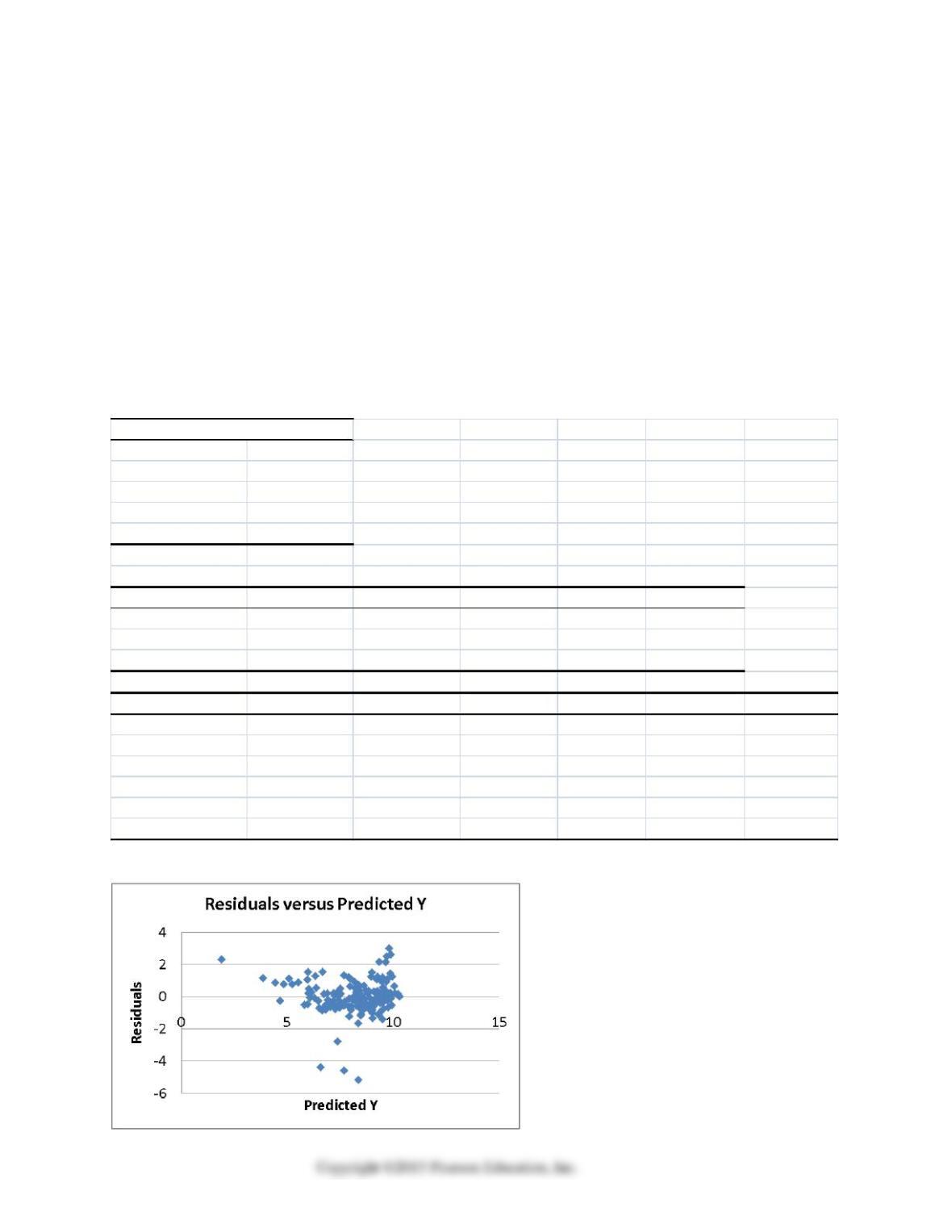
18-62 A Roadmap for Analyzing Data
SCENARIO 18-9
What are the factors that determine the acceleration time (in sec.) from 0 to 60 miles per hour of a
car? Data on the following variables for 171 different vehicle models were collected:
Accel Time: Acceleration time in sec.
Cargo Vol: Cargo volume in cu. ft.
HP: Horsepower
MPG: Miles per gallon
SUV: 1 if the vehicle model is an SUV with Coupe as the base when SUV and Sedan are both 0
Sedan: 1 if the vehicle model is a sedan with Coupe as the base when SUV and Sedan are both 0
The regression results using acceleration time as the dependent variable and the remaining variables
as the independent variables are presented below.
Re g ressio n S ta tistics
Mu lti p l e R 0.8013
R S q u are 0.6421
A d ju ste d R Sq u are 0.6313
Stan d ard Erro r 1.0507
O b s e rv ati o n s 171
A N O V A
df SS MS F Sig n if ica n ce F
Regression 5 326.8700 65.3740 59.2168 0.0000
R e s id u al 165 182.1564 1.1040
To ta l 170 509.0263
C o efficien ts Sta n d a rd Erro r t S ta t P –v a lu e Lo w er 95% U p p er 95%
Inte rce pt 12.8627 1.0927 11.7713 0.0000 10.7052 15.0202
Cargo Vol 0.0259 0.0102 2.5518 0.0116 0.0059 0.0460
HP –0.0200 0.0018 –11.3307 0.0000 -0.0235 –0.0165
MPG –0.0620 0.0303 –2.0464 0.0423 –0.1218 –0.0022
SUV 0.7679 0.4314 1.7802 0.0769 -0.0838 1.6196
Sedan 0.6427 0.2790 2.3034 0.0225 0.0918 1.1935
The various residual plots are as shown below.
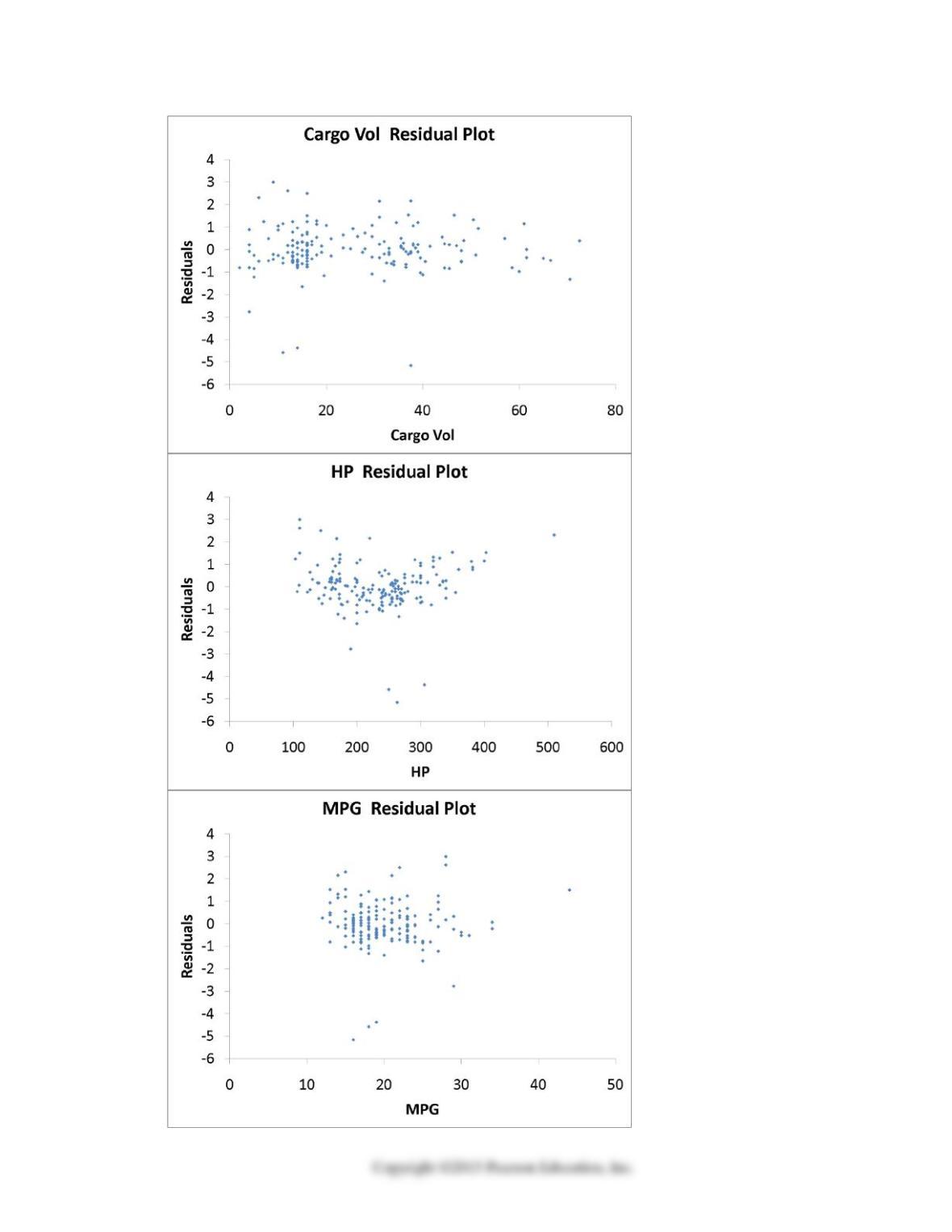
A Roadmap for Analyzing Data 18-63
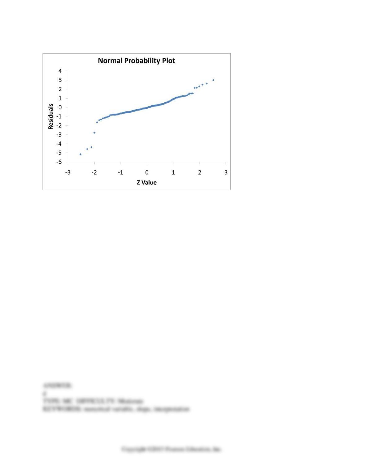
18-64 A Roadmap for Analyzing Data
The coefficient of partial determination (
2
. All variables except Yj j
R
) of each of the 5 predictors are,
respectively, 0.0380, 0.4376, 0.0248, 0.0188, and 0.0312.
The coefficient of multiple determination for the regression model using each of the 5 variables
j
X
as the dependent variable and all other X variables as independent variables (
2
j
R
) are, respectively,
0.7461, 0.5676, 0.6764, 0.8582, 0.6632.
188. Referring to Scenario 18-9, what is the correct interpretation for the estimated coefficient for
Cargo Vol?
a) As the 0 to 60 miles per hour acceleration time increases by one second, the mean cargo
volume will increase by an estimated 0.0259 cubic foot without taking into consideration
all the other independent variables included in the model.
b) As the cargo volume increases by one cubic foot, the mean 0 to 60 miles per hour
acceleration time will increase by an estimated 0.0259 seconds without taking into
consideration all the other independent variables included in the model.
c) As the 0 to 60 miles per hour acceleration time increases by one second, the mean cargo
volume will increase by an estimated 0.0259 cubic foot taking into consideration all the
other independent variables included in the model.
d) As the cargo volume increases by one cubic foot, the mean 0 to 60 miles per hour
acceleration time will increase by an estimated 0.0259 seconds taking into consideration
all the other independent variables included in the model.

A Roadmap for Analyzing Data 18-65
189. Referring to Scenario 18-9, what is the correct interpretation for the estimated coefficient for
HP?
a) As the horsepower increases by one unit, the mean 0 to 60 miles per hour acceleration
time will decrease by an estimated 0.0200 seconds without taking into consideration all
the other independent variables included in the model.
b) As the 0 to 60 miles per hour acceleration time increases by one second, the mean
horsepower will decrease by an estimated 0.0200 unit without taking into consideration
all the other independent variables included in the model.
c) As the horsepower increases by one unit, the mean 0 to 60 miles per hour acceleration
time will decrease by an estimated 0.0200 seconds taking into consideration all the other
independent variables included in the model.
d) As the 0 to 60 miles per hour acceleration time increases by one second, the mean
horsepower will decrease by an estimated 0.0200 unit taking into consideration all the
other independent variables included in the model.
190. Referring to Scenario 18-9, what is the correct interpretation for the estimated coefficient for
MPG?
a) As the miles per gallon decreases by one unit, the mean 0 to 60 miles per hour
acceleration time will increase by an estimated 0.0620 seconds without taking into
consideration all the other independent variables included in the model.
b) As the 0 to 60 miles per hour acceleration time decreases by one second, the mean miles
per gallon will increase by an estimated 0.0620 unit without taking into consideration all
the other independent variables included in the model.
c) As the miles per gallon decreases by one unit, the mean 0 to 60 miles per hour
acceleration time will increase by an estimated 0.0620 seconds taking into consideration
all the other independent variables included in the model.
d) As the 0 to 60 miles per hour acceleration time decreases by one second, the mean miles
per gallon will increase by an estimated 0.0620 unit taking into consideration all the
other independent variables included in the model.

18-66 A Roadmap for Analyzing Data
191. Referring to Scenario 18-9, what is the correct interpretation for the estimated coefficient for
SUV?
a) The mean 0 to 60 miles per hour acceleration time of an SUV is estimated to be 0.7679
seconds higher than that of a coupe after considering the effect of all the other
independent variables in the model.
b) The mean 0 to 60 miles per hour acceleration time of an SUV is estimated to be 0.7679
seconds higher than that of a sedan after considering the effect of all the other
independent variables in the model.
c) The mean 0 to 60 miles per hour acceleration time of an SUV is estimated to be 0.7679
seconds lower than that of a coupe after considering the effect of all the other
independent variables in the model.
d) The mean 0 to 60 miles per hour acceleration time of an SUV is estimated to be 0.7679
seconds lower than that of a sedan after considering the effect of all the other
independent variables in the model.
192. Referring to Scenario 18-9, what is the correct interpretation for the estimated coefficient for
Sedan?
a) The mean 0 to 60 miles per hour acceleration time of a sedan is estimated to be 0.6427
seconds higher than that of a coupe after considering the effect of all the other
independent variables in the model.
b) The mean 0 to 60 miles per hour acceleration time of a sedan is estimated to be 0.6427
seconds higher than that of an SUV after considering the effect of all the other
independent variables in the model.
c) The mean 0 to 60 miles per hour acceleration time of a sedan is estimated to be 0.6427
seconds lower than that of a coupe after considering the effect of all the other
independent variables in the model.
d) The mean 0 to 60 miles per hour acceleration time of a sedan is estimated to be 0.6427
seconds lower than that of an SUV after considering the effect of all the other
independent variables in the model.
193. True or False: Referring to Scenario 18-9, the 0 to 60 miles per hour acceleration time of a
sedan is predicted to be 0.1252 seconds higher than that of an SUV.

A Roadmap for Analyzing Data 18-67
194. True or False: Referring to Scenario 18-9, the 0 to 60 miles per hour acceleration time of an
SUV is predicted to be 0.1252 seconds higher than that of a sedan.
195. True or False: Referring to Scenario 18-9, the 0 to 60 miles per hour acceleration time of a
coupe is predicted to be 0.6427 seconds lower than that of a sedan.
196. True or False: Referring to Scenario 18-9, the 0 to 60 miles per hour acceleration time of a
coupe is predicted to be 0.7679 seconds lower than that of an SUV.
197. True or False: Referring to Scenario 18-9, the 0 to 60 miles per hour acceleration time of a
coupe is predicted to be 0.7679 seconds higher than that of a sedan.
198. True or False: Referring to Scenario 18-9, the 0 to 60 miles per hour acceleration time of a
sedan is predicted to be 0.7679 seconds higher than that of an SUV.
199. True or False: Referring to Scenario 18-9, the 0 to 60 miles per hour acceleration time of a
sedan is predicted to be 0.6427 seconds higher than that of an SUV.
18-68 A Roadmap for Analyzing Data
200. Referring to Scenario 18-9, what is the value of the test statistic to determine whether Cargo
Vol makes a significant contribution to the regression model in the presence of the other
independent variables at a 5% level of significance?
201. Referring to Scenario 18-9, what is the p-value of the test statistic to determine whether Cargo
Vol makes a significant contribution to the regression model in the presence of the other
independent variables at a 5% level of significance?
202. True or False: Referring to Scenario 18-9, there is enough evidence to conclude that Cargo Vol
makes a significant contribution to the regression model in the presence of the other independent
variables at a 5% level of significance.
203. Referring to Scenario 18-9, what is the value of the test statistic to determine whether HP
makes a significant contribution to the regression model in the presence of the other independent
variables at a 5% level of significance?
204. Referring to Scenario 18-9, what is the p-value of the test statistic to determine whether HP
makes a significant contribution to the regression model in the presence of the other independent
variables at a 5% level of significance?
A Roadmap for Analyzing Data 18-69
205. True or False: Referring to Scenario 18-9, there is enough evidence to conclude that HP makes
a significant contribution to the regression model in the presence of the other independent
variables at a 5% level of significance.
206. Referring to Scenario 18-9, what is the value of the test statistic to determine whether MPG
makes a significant contribution to the regression model in the presence of the other independent
variables at a 5% level of significance?
207. Referring to Scenario 18-9, what is the p-value of the test statistic to determine whether MPG
makes a significant contribution to the regression model in the presence of the other independent
variables at a 5% level of significance?
208. True or False: Referring to Scenario 18-9, there is enough evidence to conclude that MPG
makes a significant contribution to the regression model in the presence of the other independent
variables at a 5% level of significance.
209. Referring to Scenario 18-9, what is the value of the test statistic to determine whether SUV
makes a significant contribution to the regression model in the presence of the other independent
variables at a 5% level of significance?
18-70 A Roadmap for Analyzing Data
210. Referring to Scenario 18-9, what is the p-value of the test statistic to determine whether SUV
makes a significant contribution to the regression model in the presence of the other independent
variables at a 5% level of significance?
211. True or False: Referring to Scenario 18-9, there is enough evidence to conclude that SUV
makes a significant contribution to the regression model in the presence of the other independent
variables at a 5% level of significance.
212. Referring to Scenario 18-9, ________ of the variation in Accel Time can be explained by the
five independent variables after taking into consideration the number of independent variables
and the number of observations.
213. Referring to Scenario 18-9, ________ of the variation in Accel Time can be explained by the
five independent variables.
214. Referring to Scenario 18-9, ________ of the variation in Accel Time can be explained by
Cargo Vol while controlling for the other independent variables.
215. Referring to Scenario 18-9, ________ of the variation in Accel Time can be explained by HP
while controlling for the other independent variables.

A Roadmap for Analyzing Data 18-71
216. Referring to Scenario 18-9, ________ of the variation in Accel Time can be explained by MPG
while controlling for the other independent variables.
217. Referring to Scenario 18-9, which of the following assumptions is most likely violated based
on the residual plot of the residuals versus predicted Y?
a) Independence of errors.
b) Normality of errors.
c) Equal variance.
d) None.
218. Referring to Scenario 18-9, which of the following assumptions is most likely violated based
on the residual plot for HP?
a) Linearity.
b) Normality of errors.
c) Independence of errors.
d) None.
219. Referring to Scenario 18-9, which of the following assumptions is most likely violated based
on the normal probability plot?
a) Linearity.
b) Normality of errors.
c) Equal variance.
d) None.
220. True or False: Referring to Scenario 18-9, the error appears to be left-skewed.

18-72 A Roadmap for Analyzing Data
221. True or False: Referring to Scenario 18-9, the errors (residuals) appear to be right-skewed.
222. True or False: Referring to Scenario 18-9, the errors (residuals) appear to be normally
distributed.

A Roadmap for Analyzing Data 18-73
SCENARIO 18-10
Given below are results from the regression analysis where the dependent variable is the number of
weeks a worker is unemployed due to a layoff (Unemploy) and the independent variables are the age
of the worker (Age), the number of years of education received (Edu), the number of years at the
previous job (Job Yr), a dummy variable for marital status (Married: 1 = married, 0 = otherwise), a
dummy variable for head of household (Head: 1 = yes, 0 = no) and a dummy variable for
management position (Manager: 1 = yes, 0 = no). We shall call this Model 1. The coefficient of
partial determination (
2
. All variables except Yj j
R
) of each of the 6 predictors are, respectively, 0.2807,
0.0386, 0.0317, 0.0141, 0.0958, and 0.1201.
Regression Statistics
Multiple R
0.7035
R Square
0.4949
Adjusted R
Square
0.4030
Standard
Error
18.4861
Observations
40
ANOVA
df
SS
MS
F
Significance F
Regression
6
11048.6415
1841.4402
5.3885
0.00057
Residual
33
11277.2586
341.7351
Total
39
22325.9
Coefficients
Standard Error
t Stat
P-value
Lower 95%
Upper 95%
Intercept
32.6595
23.18302
1.4088
0.1683
-14.5067
79.8257
Age
1.2915
0.3599
3.5883
0.0011
0.5592
2.0238
Edu
-1.3537
1.1766
-1.1504
0.2582
-3.7476
1.0402
Job Yr
0.6171
0.5940
1.0389
0.3064
-0.5914
1.8257
Married
-5.2189
7.6068
-0.6861
0.4974
-20.6950
10.2571
Head
-14.2978
7.6479
-1.8695
0.0704
-29.8575
1.2618
Manager
-24.8203
11.6932
-2.1226
0.0414
-48.6102
-1.0303

18-74 A Roadmap for Analyzing Data
Model 2 is the regression analysis where the dependent variable is Unemploy and the independent
variables are Age and Manager. The results of the regression analysis are given below:
Regression Statistics
Multiple R
0.6391
R Square
0.4085
Adjusted R
Square
0.3765
Standard Error
18.8929
Observations
40
ANOVA
df
SS
MS
F
Significance F
Regression
2
9119.0897
4559.5448
12.7740
0.0000
Residual
37
13206.8103
356.9408
Total
39
22325.9
Coefficients
Standard Error
t Stat
P-value
Intercept
-0.2143
11.5796
-0.0185
0.9853
Age
1.4448
0.3160
4.5717
0.000
0
Manager
-22.5761
11.3488
-1.9893
0.0541
223. Referring to Scenario 18-10 Model 1, which of the following is a correct statement?
a) On average, a worker who is a year older is estimated to stay jobless longer by
approximately 32.66 weeks while holding constant the effects of all the remaining
independent variables.
b) On average, a worker who is a year older is estimated to stay jobless longer by
approximately 1.29 weeks while holding constant the effects of all the remaining
independent variables.
c) On average, a worker who is a year older is estimated to stay jobless shorter by
approximately 1.35 weeks while holding constant the effects of all the remaining
independent variables.
d) On average, a worker who is a year older is estimated to stay jobless longer by
approximately 0.62 weeks while holding constant the effects of all the remaining
independent variables.

A Roadmap for Analyzing Data 18-75
224. Referring to Scenario 18-10 Model 1, which of the following is a correct statement?
a) On average, those who are in a management position are estimated to stay jobless shorter
by approximately 1.35 weeks while holding constant the effects of all the remaining
independent variables.
b) On average, those who are in a management position are estimated to stay jobless shorter
by approximately 5.22 weeks while holding constant the effects of all the remaining
independent variables.
c) On average, those who are in a management position are estimated to stay jobless shorter
by approximately 14.30 weeks while holding constant the effects of all the remaining
independent variables.
d) On average, those who are in a management position are estimated to stay jobless shorter
by approximately 24.82 weeks while holding constant the effects of all the remaining
independent variables.
225. Referring to Scenario 18-10 Model 1, which of the following is a correct statement?
a) 49.49% of the total variation in the number of weeks a worker is unemployed due to a
layoff can be explained by the age of the worker, the number of years of education
received, the number of years at the previous job, marital status, whether the worker is
the head of household and whether the worker is a manager.
b) 49.49% of the total variation in the number of weeks a worker is unemployed due to a
layoff can be explained by the age of the worker, the number of years of education
received, the number of years at the previous job, marital status, whether the worker is
the head of household and whether the worker is a manager after adjusting for the
number of predictors and sample size.
c) 49.49% of the total variation in the number of weeks a worker is unemployed due to a
layoff can be explained by the age of the worker, the number of years of education
received, the number of years at the previous job, marital status, whether the worker is
the head of household and whether the worker is a manager after adjusting for the level
of significance
d) 49.49% of the total variation in the number of weeks a worker is unemployed due to a
layoff can be explained by the age of the worker, the number of years of education
received, the number of years at the previous job, marital status, whether the worker is
the head of household and whether the worker is a manager holding constant the effect of
all the independent variables.

18-76 A Roadmap for Analyzing Data
226. Referring to Scenario 18-10 Model 1, which of the following is a correct statement?
a) 40.30% of the total variation in the number of weeks a worker is unemployed due to a
layoff can be explained by the age of the worker, the number of years of education
received, the number of years at the previous job, marital status, whether the worker is
the head of household and whether the worker is a manager.
b) 40.30% of the total variation in the number of weeks a worker is unemployed due to a
layoff can be explained by the age of the worker, the number of years of education
received, the number of years at the previous job, marital status, whether the worker is
the head of household and whether the worker is a manager after adjusting for the
number of predictors and sample size.
c) 40.30% of the total variation in the number of weeks a worker is unemployed due to a
layoff can be explained by the age of the worker, the number of years of education
received, the number of years at the previous job, marital status, whether the worker is
the head of household and whether the worker is a manager after adjusting for the level
of significance
d) 40.30% of the total variation in the number of weeks a worker is unemployed due to a
layoff can be explained by the age of the worker, the number of years of education
received, the number of years at the previous job, marital status, whether the worker is
the head of household and whether the worker is a manager holding constant the effect of
all the independent variables.
227. Referring to Scenario 18-10 Model 1, what is the standard error of estimate?
228. Referring to Scenario 18-10 Model 1, predict the number of weeks being unemployed due to a
layoff for a worker who is a thirty-year old, has 10 years of education, has 15 years of experience
at the previous job, is married, is the head of household and is a manager.
229. Referring to Scenario 18-10 Model 1, estimate the mean number of weeks being unemployed
due to a layoff for a worker who is a thirty-year old, has 10 years of education, has 15 years of
experience at the previous job, is married, is the head of household and is a manager.

A Roadmap for Analyzing Data 18-77
230. Referring to Scenario 18-10 Model 1, which of the following is the correct null hypothesis to
test whether being married or not makes a difference in the mean number of weeks a worker is
unemployed due to a layoff while holding constant the effect of all the other independent
variables?
a)
01
:0H
b)
02
:0H
c)
03
:0H
d)
04
:0H
231. Referring to Scenario 18-10 Model 1, which of the following is the correct alternative
hypothesis to test whether being married or not makes a difference in the mean number of weeks
a worker is unemployed due to a layoff while holding constant the effect of all the other
independent variables?
a)
11
:0H
b)
12
:0H
c)
13
:0H
d)
14
:0H
232. Referring to Scenario 18-10 Model 1, what is the value of the test statistic when testing
whether being married or not makes a difference in the mean number of weeks a worker is
unemployed due to a layoff while holding constant the effect of all the other independent
variables?
233. Referring to Scenario 18-10 Model 1, what is the p-value of the test statistic when testing
whether being married or not makes a difference in the mean number of weeks a worker is
unemployed due to a layoff while holding constant the effect of all the other independent
variables?

18-78 A Roadmap for Analyzing Data
234. True or False: Referring to Scenario 18-10 Model 1, the null hypothesis should be rejected at a
10% level of significance when testing whether being married or not makes a difference in the
mean number of weeks a worker is unemployed due to a layoff while holding constant the effect
of all the other independent variables.
235. True or False: Referring to Scenario 18-10 Model 1, there is sufficient evidence that being
married or not makes a difference in the mean number of weeks a worker is unemployed due to a
layoff while holding constant the effect of all the other independent variables at a 10% level of
significance.
236. Referring to Scenario 18-10 Model 1, which of the following is the correct null hypothesis to
test whether age has any effect on the number of weeks a worker is unemployed due to a layoff
while holding constant the effect of all the other independent variables?
a)
00
:0H
b)
01
:0H
c)
02
:0H
d)
03
:0H
237. Referring to Scenario 18-10 Model 1, which of the following is the correct alternative
hypothesis to test whether age has any effect on the number of weeks a worker is unemployed
due to a layoff while holding constant the effect of all the other independent variables?
a)
10
:0H
b)
11
:0H
c)
12
:0H
d)
13
:0H

A Roadmap for Analyzing Data 18-79
238. Referring to Scenario 18-10 Model 1, what is the value of the test statistic when testing
whether age has any effect on the number of weeks a worker is unemployed due to a layoff while
holding constant the effect of all the other independent variables?
239. Referring to Scenario 18-10 Model 1, what is the p-value of the test statistic when testing
whether age has any effect on the number of weeks a worker is unemployed due to a layoff while
holding constant the effect of all the other independent variables?
240. True or False: Referring to Scenario 18-10 Model 1, the null hypothesis should be rejected at a
10% level of significance when testing whether age has any effect on the number of weeks a
worker is unemployed due to a layoff.
241. True or False: Referring to Scenario 18-10 Model 1, there is sufficient evidence that age has an
effect on the number of weeks a worker is unemployed due to a layoff while holding constant the
effect of all the other independent variables at a 10% level of significance.
242. Referring to Scenario 18-10 Model 1, which of the following is the correct null hypothesis to
determine whether there is a significant relationship between the number of weeks a worker is
unemployed due to a layoff and the entire set of explanatory variables?
a)
0 0 1 2 3 4 5 6
:0H
b)
0123456
:0H
c)
0 0 1 2 3 4 5 6
:H
d)
0123456
:H

18-80 A Roadmap for Analyzing Data
243. Referring to Scenario 18-10 Model 1, which of the following is the correct alternative
hypothesis to determine whether there is a significant relationship between the number of weeks
a worker is unemployed due to a layoff and the entire set of explanatory variables?
a)
1:H
All
0
j
for j = 0, 1, 2, 3, 4, 5, 6
b)
1:H
All
0
j
for j = 1, 2, 3, 4, 5, 6
c)
1:H
At least one of
0
j
for j = 0, 1, 2, 3, 4, 5, 6
d)
1:H
At least one of
0
j
for j = 1, 2, 3, 4, 5, 6
244. Referring to Scenario 18-10 Model 1 Model 1, the null hypothesis
0123456
:0H
implies that the number of weeks a worker is
unemployed due to a layoff is not affected by any of the explanatory variables.
245. Referring to Scenario 18-10 Model 1, the null hypothesis
0123456
:0H
implies that the number of weeks a worker is
unemployed due to a layoff is not affected by some of the explanatory variables.
246. Referring to Scenario 18-10 Model 1, the null hypothesis
0123456
:0H
implies that the number of weeks a worker is
unemployed due to a layoff is not related to any of the explanatory variables.

A Roadmap for Analyzing Data 18-81
247. Referring to Scenario 18-10 Model 1, the null hypothesis
0123456
:0H
implies that the number of weeks a worker is
unemployed due to a layoff is not related to one of the explanatory variables.
248. Referring to Scenario 18-10 Model 1, the alternative hypothesis
1:H
At least one of
0
j
for j = 1, 2, 3, 4, 5, 6 implies that the number of weeks a worker is unemployed due to a layoff is
related to all of the explanatory variables.
249. Referring to Scenario 18-10 Model 1, the alternative hypothesis
1:H
At least one of
0
j
for j = 1, 2, 3, 4, 5, 6 implies that the number of weeks a worker is unemployed due to a layoff is
related to at least one of the explanatory variables.
250. Referring to Scenario 18-10 Model 1, the alternative hypothesis
1:H
At least one of
0
j
for j = 1, 2, 3, 4, 5, 6 implies that the number of weeks a worker is unemployed due to a layoff is
affected by all of the explanatory variables.
251. Referring to Scenario 18-10 Model 1, the alternative hypothesis
1:H
At least one of
0
j
for j = 1, 2, 3, 4, 5, 6 implies that the number of weeks a worker is unemployed due to a layoff is
affected by at least one of the explanatory variables.
18-82 A Roadmap for Analyzing Data
252. Referring to Scenario 18-10 Model 1, what are the numerator and denominator degrees of
freedom, respectively, for the test statistic to determine whether there is a significant relationship
between the number of weeks a worker is unemployed due to a layoff and the entire set of
explanatory variables?
253. Referring to Scenario 18-10 Model 1, what is the value of the test statistic to determine
whether there is a significant relationship between the number of weeks a worker is unemployed
due to a layoff and the entire set of explanatory variables?
254. Referring to Scenario 18-10 Model 1, what is the p-value of the test statistic to determine
whether there is a significant relationship between the number of weeks a worker is unemployed
due to a layoff and the entire set of explanatory variables?
255. True or False: Referring to Scenario 18-10 Model 1, the null hypothesis should be rejected at a
10% level of significance when testing whether there is a significant relationship between the
number of weeks a worker is unemployed due to a layoff and the entire set of explanatory
variables.
256. True or False: Referring to Scenario 18-10 Model 1, there is sufficient evidence that at least
one of the explanatory variables is related to the number of weeks a worker is unemployed due to
a layoff at a 10% level of significance.

A Roadmap for Analyzing Data 18-83
257. True or False: Referring to Scenario 18-10 Model 1, there is sufficient evidence that the
number of weeks a worker is unemployed due to a layoff depends on at least one of the
explanatory variables at a 10% level of significance.
258. True or False: Referring to Scenario 18-10 Model 1, there is sufficient evidence that all of the
explanatory variables are related to the number of weeks a worker is unemployed due to a layoff
at a 10% level of significance.
259. True or False: Referring to Scenario 18-10 Model 1, there is sufficient evidence that the
number of weeks a worker is unemployed due to a layoff depends on all of the explanatory
variables at a 10% level of significance.
260. Referring to Scenario 18-10 Model 1, what are the lower and upper limits of the 95%
confidence interval estimate for the effect of a one year increase in education received on the
mean number of weeks a worker is unemployed due to a layoff after taking into consideration the
effect of all the other independent variables?
261. Referring to Scenario 18-10 Model 1, what are the lower and upper limits of the 95%
confidence interval estimate for the difference in the mean number of weeks a worker is
unemployed due to a layoff between a worker who is married and one who is not after taking into
consideration the effect of all the other independent variables?
18-84 A Roadmap for Analyzing Data
262. True or False: Referring to Scenario 18-10 Model 1, you can conclude that, holding constant
the effect of the other independent variables, the number of years of education received has no
impact on the mean number of weeks a worker is unemployed due to a layoff at a 5% level of
significance if we use only the information of the 95% confidence interval estimate for
2
.
263. True or False: Referring to Scenario 18-10 Model 1, we can conclude that, holding constant the
effect of the other independent variables, there is a difference in the mean number of weeks a
worker is unemployed due to a layoff between a worker who is married and one who is not at a
5% level of significance if we use only the information of the 95% confidence interval estimate
for
4
.
264. True or False: Referring to Scenario 18-10 Model 1, we can conclude that, holding constant the
effect of the other independent variables, the number of years of education received has no
impact on the mean number of weeks a worker is unemployed due to a layoff at a 1% level of
significance if all we have is the information of the 95% confidence interval estimate for
2
.
A Roadmap for Analyzing Data 18-85
265. True or False: Referring to Scenario 18-10 Model 1, we can conclude that, holding constant the
effect of the other independent variables, there is a difference in the mean number of weeks a
worker is unemployed due to a layoff between a worker who is married and one who is not at a
1% level of significance if all we have is the information of the 95% confidence interval estimate
for
4
.
4
266. True or False: Referring to Scenario 18-10 Model 1, we can conclude that, holding constant the
effect of the other independent variables, the number of years of education received has no
impact on the mean number of weeks a worker is unemployed due to a layoff at a 10% level of
significance if all we have is the information on the 95% confidence interval estimate for
2
.
267. True or False: Referring to Scenario 18-10 Model 1, we can conclude that, holding constant the
effect of the other independent variables, there is a difference in the mean number of weeks a
worker is unemployed due to a layoff between a worker who is married and one who is not at a
10% level of significance if we use only the information of the 95% confidence interval estimate
for
4
.
4

18-86 A Roadmap for Analyzing Data
268. Referring to Scenario 18-10 Model 1, which of the six independent variables (Age, Edu, Job
Yr, Married, Head and Manager) is (are) insignificant in affecting the dependent variable using a
5% level of significance after taking into account the effect of the remaining independent
variables?
269. Referring to Scenario 18-10 Model 1, ________ of the variation in the number of weeks a
worker is unemployed due to a layoff can be explained by the six independent variables after
taking into consideration the number of independent variables and the number of observations.
270. Referring to Scenario 18-10 Model 1, ________ of the variation in the number of weeks a
worker is unemployed due to a layoff can be explained by the six independent variables.
271. Referring to Scenario 18-10 Model 1, ________ of the variation in the number of weeks a
worker is unemployed due to a layoff can be explained by the age of the worker while controlling
for the other independent variables.
272. Referring to Scenario 18-10 Model 1, ________ of the variation in the number of weeks a
worker is unemployed due to a layoff can be explained by the number of years of education
received while controlling for the other independent variables.

A Roadmap for Analyzing Data 18-87
273. Referring to Scenario 18-10 Model 1, ________ of the variation in the number of weeks a
worker is unemployed due to a layoff can be explained by the number of years at the previous job
while controlling for the other independent variables.
274. Referring to Scenario 18-10 Model 1, ________ of the variation in the number of weeks a
worker is unemployed due to a layoff can be explained by the marital status while controlling for
the other independent variables.
275. Referring to Scenario 18-10 Model 1, ________ of the variation in the number of weeks a
worker is unemployed due to a layoff can be explained by whether the worker is head of
household while controlling for the other independent variables.
276. Referring to Scenario 18-10 Model 1, ________ of the variation in the number of weeks a
worker is unemployed due to a layoff can be explained by whether the worker is in a
management position while controlling for the other independent variables.
277. Referring to Scenario 18-10 and using both Model 1 and Model 2, what are the null and
alternative hypotheses for testing whether the independent variables that are not significant
individually are also not significant as a group in explaining the variation in the dependent
variable at a 5% level of significance?
18-88 A Roadmap for Analyzing Data
278. Referring to Scenario 18-10 and using both Model 1 and Model 2, what are the degrees of
freedom of the test statistic for testing whether the independent variables that are not significant
individually are also not significant as a group in explaining the variation in the dependent
variable at a 5% level of significance?
279. Referring to Scenario 18-10 and using both Model 1 and Model 2, what is the value of the test
statistic for testing whether the independent variables that are not significant individually are also
not significant as a group in explaining the variation in the dependent variable at a 5% level of
significance?
341.7351075
280. Referring to Scenario 18-10 and using both Model 1 and Model 2, what is the p-value of the
test statistic for testing whether the independent variables that are not significant individually are
also not significant as a group in explaining the variation in the dependent variable at a 5% level
of significance?
281. Referring to Scenario 18-10 and using both Model 1 and Model 2, what is the critical value of
the test statistic for testing whether the independent variables that are not significant individually
are also not significant as a group in explaining the variation in the dependent variable at a 5%
level of significance?

A Roadmap for Analyzing Data 18-89
282. True or False: Referring to Scenario 18-10 and using both Model 1 and Model 2, the null
hypothesis for testing whether the independent variables that are not significant individually are
also not significant as a group in explaining the variation in the dependent variable should be
rejected at a 5% level of significance?
283. True or False: Referring to Scenario 18-10 and using both Model 1 and Model 2, there is
sufficient evidence to conclude that the independent variables that are not significant individually
are also not significant as a group in explaining the variation in the dependent variable at a 5%
level of significance?
284. True or False: Referring to Scenario 18-10 and using both Model 1 and Model 2, there is
insufficient evidence to conclude that the independent variables that are not significant
individually are significant as a group in explaining the variation in the dependent variable at a
5% level of significance?
285. True or False: Referring to Scenario 18-10 and using both Model 1 and Model 2, there is
sufficient evidence to conclude that at least one of the independent variables that are not
significant individually has become significant as a group in explaining the variation in the
dependent variable at a 5% level of significance?

18-90 A Roadmap for Analyzing Data
SCENARIO 18-11
A logistic regression model was estimated in order to predict the probability that a randomly chosen
university or college would be a private university using information on mean total Scholastic
Aptitude Test score (SAT) at the university or college, the room and board expense measured in
thousands of dollars (Room/Brd), and whether the TOEFL criterion is at least 550 (Toefl550 = 1 if
yes, 0 otherwise.) The dependent variable, Y, is school type (Type = 1 if private and 0 otherwise).
The Minitab output is given below:
Logistic Regression Table
Odds 95% CI
Predictor Coef SE Coef Z P Ratio Lower Upper
Constant -27.118 6.696 -4.05 0.000
SAT 0.015 0.004666 3.17 0.002 1.01 1.01 1.02
Toefl550 -0.390 0.9538 -0.41 0.682 0.68 0.10 4.39
Room/Brd 2.078 0.5076 4.09 0.000 7.99 2.95 21.60
Log-Likelihood = -21.883
Test that all slopes are zero: G = 62.083, DF = 3, P-Value = 0.000
Goodness-of-Fit Tests
Method Chi-Square DF P
Pearson 143.551 76 0.000
Deviance 43.767 76 0.999
Hosmer-Lemeshow 15.731 8 0.046
286. Referring to Scenario 18-11, which of the following is the correct expression for the estimated
model?
a)
27.118 0.015 0.390 550 2.078 /Y SAT Toefl Room Brd
b)
ˆ27.118 0.015 0.390 550 2.078 /Y SAT Toefl Room Brd
c)
ln odds ratio 27.118 0.015 0.390 550 2.078 /SAT Toefl Room Brd
d)
ln estimated odds ratio 27.118 0.015 0.390 550 2.078 /SAT Toefl Room Brd
287. Referring to Scenario 18-11, what is the estimated odds ratio for a school with an mean SAT
score of 1250, a TOEFL criterion that is at least 550, and the room and board expense of 5
thousand dollars?

A Roadmap for Analyzing Data 18-91
288. Referring to Scenario 18-11, what is the estimated probability that a school with an mean SAT
score of 1250, a TOEFL criterion that is at least 550, and the room and board expense of 5
thousand dollars will be a private school?
289. Referring to Scenario 18-11, what is the estimated odds ratio for a school with an mean SAT
score of 1100, a TOEFL criterion that is not at least 550, and the room and board expense of 7
thousand dollars?
290. Referring to Scenario 18-11, what is the estimated probability that a school with an mean SAT
score of 1100, a TOEFL criterion that is not at least 550, and the room and board expense of 7
thousand dollars will be a private school?
291. Referring to Scenario 18-11, which of the following is the correct interpretation for the SAT
slope coefficient?
a) Holding constant the effect of the other variables, the estimated mean value of school
type increases by 0.015 for each increase of one point in average SAT score.
b) Holding constant the effect of the other variables, the estimated school type increases by
0.015 for each increase of one point in average SAT score.
c) Holding constant the effect of the other variables, the estimated probability of the school
being a private school increases by 0.015 for each increase of one point in mean SAT
score.
d) Holding constant the effect of the other variables, the estimated natural logarithm of the
odds ratio of the school being a private school increases by 0.015 for each increase of
one point in mean SAT score.

18-92 A Roadmap for Analyzing Data
292. Referring to Scenario 18-11, which of the following is the correct interpretation for the
Tofel500 slope coefficient?
a) Holding constant the effect of the other variables, the estimated mean value of school
type is 0.39 lower when the school has a TOEFL criterion that is at least 550.
b) Holding constant the effect of the other variables, the estimated school type decreases by
0.39 when the school has a TOEFL criterion that is at least 550.
c) Holding constant the effect of the other variables, the estimated natural logarithm of the
odds ratio of the school being a private school is 0.39 lower for a school that has a
TOEFL criterion that is at least 550 than one that does not.
d) Holding constant the effect of the other variables, the estimated probability of the school
being a private school is 0.39 lower for a school that has a TOEFL criterion that is at
least 550 than one that does not.
293. Referring to Scenario 18-11, what are the degrees of freedom for the chi-square distribution
when testing whether the model is a good-fitting model?
294. Referring to Scenario 18-11, what is the p-value of the test statistic when testing whether the
model is a good-fitting model?
295. True or False: Referring to Scenario 18-11, the null hypothesis that the model is a good-fitting
model cannot be rejected when allowing for a 5% probability of making a type I error.
296. True or False: Referring to Scenario 18-11, there is not enough evidence to conclude that the
model is not a good-fitting model at a 0.05 level of significance.

A Roadmap for Analyzing Data 18-93
297. Referring to Scenario 18-11, what is the p-value of the test statistic when testing whether SAT
makes a significant contribution to the model in the presence of the other independent variables?
298. Referring to Scenario 18-11, what should be the decision (‘reject’ or ‘do not reject’) on the null
hypothesis when testing whether SAT makes a significant contribution to the model in the
presence of the other independent variables at a 0.05 level of significance?
299. True or False: Referring to Scenario 18-11, there is not enough evidence to conclude that SAT
score makes a significant contribution to the model in the presence of the other independent
variables at a 0.05 level of significance.
300. Referring to Scenario 18-11, what is the p-value of the test statistic when testing whether
Toefl500 makes a significant contribution to the model in the presence of the other independent
variables?
301. Referring to Scenario 18-11, what should be the decision (‘reject’ or ‘do not reject’) on the null
hypothesis when testing whether Toefl500 makes a significant contribution to the model in the
presence of the other independent variables at a 0.05 level of significance?

18-94 A Roadmap for Analyzing Data
302. True or False: Referring to Scenario 18-11, there is not enough evidence to conclude that
Toefl500 makes a significant contribution to the model in the presence of the other independent
variables at a 0.05 level of significance.
SCENARIO 18-12
The marketing manager for a nationally franchised lawn service company would like to study the
characteristics that differentiate home owners who do and do not have a lawn service. A random
sample of 30 home owners located in a suburban area near a large city was selected; 15 did not have
a lawn service (code 0) and 15 had a lawn service (code 1). Additional information available
concerning these 30 home owners includes family income (Income, in thousands of dollars), lawn
size (Lawn Size, in thousands of square feet), attitude toward outdoor recreational activities (Atitude
0 = unfavorable, 1 = favorable), number of teenagers in the household (Teenager), and age of the
head of the household (Age).
The Minitab output is given below:
Logistic Regression Table
Odds 95% CI
Predictor Coef SE Coef Z P Ratio Lower Upper
Constant -70.49 47.22 -1.49 0.135
Income 0.2868 0.1523 1.88 0.060 1.33 0.99 1.80
LawnSiz 1.0647 0.7472 1.42 0.154 2.90 0.67 12.54
Attitude -12.744 9.455 -1.35 0.178 0.00 0.00 326.06
Teenager -0.200 1.061 -0.19 0.850 0.82 0.10 6.56
Age 1.0792 0.8783 1.23 0.219 2.94 0.53 16.45
Log-Likelihood = -4.890
Test that all slopes are zero: G = 31.808, DF = 5, P-Value = 0.000
Goodness-of-Fit Tests
Method Chi-Square DF P
Pearson 9.313 24 0.997
Deviance 9.780 24 0.995
Hosmer-Lemeshow 0.571 8 1.000

A Roadmap for Analyzing Data 18-95
303. Referring to Scenario 18-12, which of the following is the correct expression for the estimated
model?
a)
AgeTeenager
AtitudeLawnSizeIncomeY
1.07920.200
12.7441.0647 0.2868 70.49
b)
AgeTeenager
AtitudeLawnSizeIncomeY
1.07920.200
12.7441.0647 0.2868 70.49
ˆ
c)
AgeTeenager
AtitudeLawnSizeIncome
1.07920.200
12.7441.0647 0.2868 70.49ratio) oddsln(
d)
AgeTeenager
AtitudeLawnSizeIncome
1.07920.200
12.7441.0647 0.2868 70.49ratio) odds estimatedln(
304. Referring to Scenario 18-12, what is the estimated odds ratio for a 48-year-old home owner
with a family income of $100,000, a lawn size of 5,000 square feet, a negative attitude toward
outdoor recreation, and one teenager in the household?
305. Referring to Scenario 18-12, what is the estimated odds ratio for a 48-year-old home owner
with a family income of $100,000, a lawn size of 5,000 square feet, a positive attitude toward
outdoor recreation, and two teenagers in the household?
306. Referring to Scenario 18-12, what is the estimated probability that a 48-year-old home owner
with a family income of $100,000, a lawn size of 5,000 square feet, a positive attitude toward
outdoor recreation, and two teenagers in the household will purchase a lawn service?

18-96 A Roadmap for Analyzing Data
307. Referring to Scenario 18-12, which of the following is the correct interpretation for the Income
slope coefficient?
a) Holding constant the effect of the other variables, the estimated number of lawn service
purchased increases by 0.2868 for each increase of one thousand dollars in family
income.
b) Holding constant the effect of the other variables, the estimated average number of lawn
service purchased increases by 0.2868 for each increase of one thousand dollars in
family income.
c) Holding constant the effect of the other variables, the estimated probability of purchasing
a lawn service increases by 0.2868 for each increase of one thousand dollars in family
income.
d) Holding constant the effect of the other variables, the estimated natural logarithm of the
odds ratio of purchasing a lawn service increases by 0.2868 for each increase of one
thousand dollars in family income.
308. Referring to Scenario 18-12, which of the following is the correct interpretation for the
Attitude slope coefficient?
a) Holding constant the effect of the other variables, the estimated number of lawn service
purchased is 12.74 lower for a home owner who has a favorable attitude toward outdoor
recreational activities than one that has an unfavorable attitude.
b) Holding constant the effect of the other variables, the estimated odds ratio of purchasing
a lawn service is 12.74 lower for a home owner who has a favorable attitude toward
outdoor recreational activities than one that has an unfavorable attitude.
c) Holding constant the effect of the other variables, the estimated natural logarithm of the
odds ratio of purchasing a lawn service is 12.74 lower for a home owner who has a
favorable attitude toward outdoor recreational activities than one that has an unfavorable
attitude.
d) Holding constant the effect of the other variables, the estimated probability of purchasing
a lawn service is 12.74 lower for a home owner who has a favorable attitude toward
outdoor recreational activities than one that has an unfavorable attitude.
309. Referring to Scenario 18-12, what are the degrees of freedom for the chi-square distribution
when testing whether the model is a good-fitting model?

A Roadmap for Analyzing Data 18-97
310. Referring to Scenario 18-12, what is the p-value of the test statistic when testing whether the
model is a good-fitting model?
311. True or False: Referring to Scenario 18-12, the null hypothesis that the model is a good-fitting
model cannot be rejected when allowing for a 5% probability of making a type I error.
312. True or False: Referring to Scenario 18-12, there is not enough evidence to conclude that the
model is not a good-fitting model at a 0.05 level of significance.
313. Referring to Scenario 18-12, what is the p-value of the test statistic when testing whether
Income makes a significant contribution to the model in the presence of the other independent
variables?
314. Referring to Scenario 18-12, what should be the decision (‘reject’ or ‘do not reject’) on the null
hypothesis when testing whether Income makes a significant contribution to the model in the
presence of the other independent variables at a 0.05 level of significance?
315. True or False: Referring to Scenario 18-12, there is not enough evidence to conclude that
Income makes a significant contribution to the model in the presence of the other independent
variables at a 0.05 level of significance.

18-98 A Roadmap for Analyzing Data
316. Referring to Scenario 18-12, what is the p-value of the test statistic when testing whether
LawnSize makes a significant contribution to the model in the presence of the other independent
variables?
317. Referring to Scenario 18-12, what should be the decision (‘reject’ or ‘do not reject’) on the null
hypothesis when testing whether LawnSize makes a significant contribution to the model in the
presence of the other independent variables at a 0.05 level of significance?
318. True or False: Referring to Scenario 18-12, there is not enough evidence to conclude that
LawnSize makes a significant contribution to the model in the presence of the other independent
variables at a 0.05 level of significance.
319. Referring to Scenario 18-12, what is the p-value of the test statistic when testing whether
Attitude makes a significant contribution to the model in the presence of the other independent
variables?
320. Referring to Scenario 18-12, what should be the decision (‘reject’ or ‘do not reject’) on the null
hypothesis when testing whether Attitude makes a significant contribution to the model in the
presence of the other independent variables at a 0.05 level of significance?

A Roadmap for Analyzing Data 18-99
321. True or False: Referring to Scenario 18-12, there is not enough evidence to conclude that
Attitude makes a significant contribution to the model in the presence of the other independent
variables at a 0.05 level of significance.
322. Referring to Scenario 18-12, what is the p-value of the test statistic when testing whether
Teenager makes a significant contribution to the model in the presence of the other independent
variables?
323. Referring to Scenario 18-12, what should be the decision (‘reject’ or ‘do not reject’) on the null
hypothesis when testing whether Teenager makes a significant contribution to the model in the
presence of the other independent variables at a 0.05 level of significance?
324. True or False: Referring to Scenario 18-12, there is not enough evidence to conclude that
Teenager makes a significant contribution to the model in the presence of the other independent
variables at a 0.05 level of significance.
325. Referring to Scenario 18-12, what is the p-value of the test statistic when testing whether Age
makes a significant contribution to the model in the presence of the other independent variables?

18-100 A Roadmap for Analyzing Data
326. Referring to Scenario 18-12, what should be the decision (‘reject’ or ‘do not reject’) on the null
hypothesis when testing whether Age makes a significant contribution to the model in the
presence of the other independent variables at a 0.05 level of significance?
327. True or False: Referring to Scenario 18-12, there is not enough evidence to conclude that Age
makes a significant contribution to the model in the presence of the other independent variables
at a 0.05 level of significance.