9. A regression model relating a dependent variable, y, with one independent variable, x1, resulted in an
SSE of 400. Another regression model with the same dependent variable, y, and two independent
variables, x1 and x2, resulted in an SSE of 320. At = .05, determine if x2 contributed significantly to
the model. The sample size for both models was 20.
10. A regression model with one independent variable, x1, resulted in an SSE of 50. When a second
independent variable, x2, was added to the model, the SSE was reduced to 40. At = 0.05, determine
if x2 contributes significantly to the model. The sample size for both models was 30.
11. When a regression model was developed relating sales (y) of a company to its product’s price (x1), the
SSE was determined to be 495. A second regression model relating sales (y) to product’s price (x1) and
competitor’s product price (x2) resulted in an SSE of 396. At = 0.05, determine if the competitor’s
product’s price contributed significantly to the model. The sample size for both models was 33.
12. A regression model relating units sold (y), price (x1), and whether or not promotion was used (x2 = 1 if
promotion was used and 0 if it was not) resulted in the following model.
= 120 – 0.03x1 + 0.7x2
and the following information is provided.
n = 15 Sb1 = .01 Sb2 = 0.1
a.
Is price a significant variable?
b.
Is promotion significant?
a.
b.
13. A regression model relating the yearly income (y), age (x1), and the gender of the faculty member of a
university (x2 = 1 if female and 0 if male) resulted in the following information.
= 5,000 + 1.2x1 + 0.9x2
n = 20 SSE = 500 SSR = 1,500
Sb1 = 0.2 Sb2 = 0.1
a.
Is gender a significant variable?
b.
Determine the multiple coefficient of determination.
14. A regression analysis was applied in order to determine the relationship between a dependent variable
and 8 independent variables. The following information was obtained from the regression analysis.
R Square = 0.80
SSR = 4,280
Total number of observations n = 56
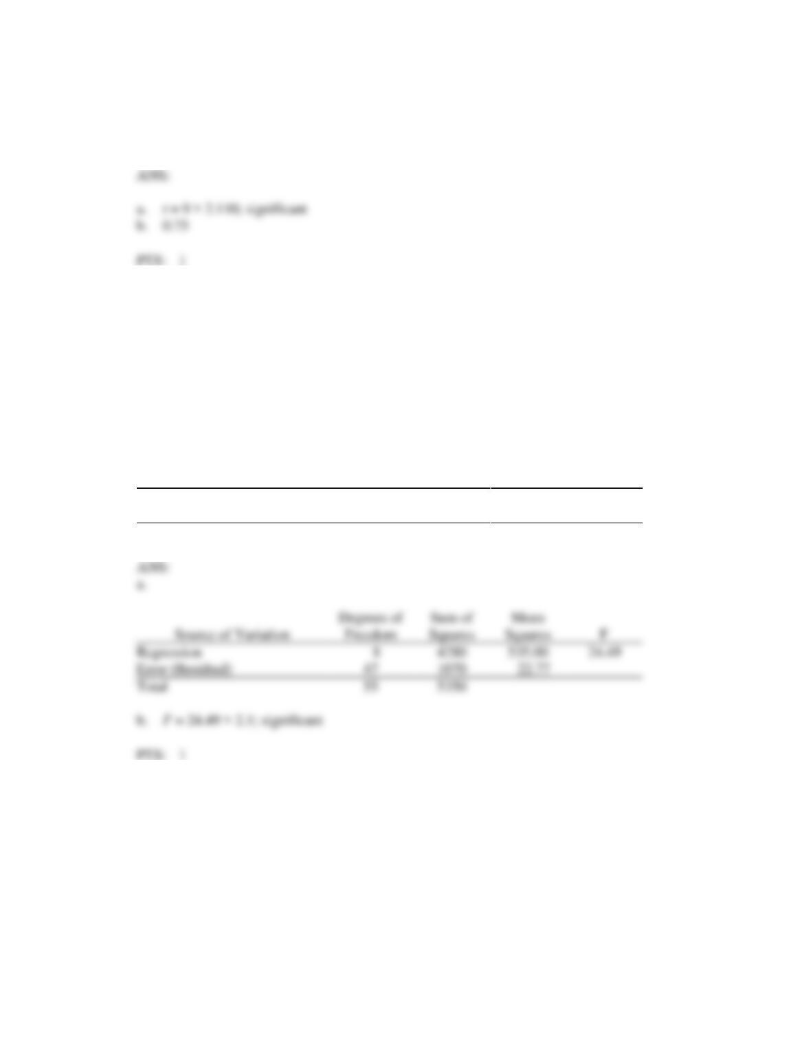
a.
Fill in the blanks in the following ANOVA table.
b.
Is the model significant? Let = 0.05.
Source of Variation
Degrees of
Freedom
Sum of
Squares
Mean
Squares
F
Regression
_____?
_____?
_____?
_____?
Error (Residual)
_____?
_____?
_____?
Total
_____?
_____?
Source of Variation
Freedom
Regression
24.49
Error (Residual)
Total
b.
15. In a regression analysis involving 18 observations and four independent variables, the following
information was obtained.
Multiple R = 0.6000
R Square = 0.3600
Standard Error = 4.8000
Based on the above information, fill in all the blanks in the following ANOVA table.
Degrees of
Sum of
Mean
a.
b.
0.75
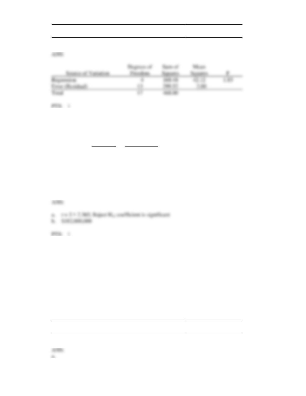
Source of Variation
Freedom
Squares
Squares
F
Regression
_____?
_____?
_____?
_____?
Error (Residual)
_____?
_____?
_____?
Total
_____?
_____?
16. The following are partial results of a regression analysis involving sales (y in millions of dollars),
advertising expenditures (x1 in thousands of dollars), and number of salespeople (x2) for a corporation.
The regression was performed on a sample of 10 observations.
Coefficient
Standard Error
Constant
50.00
20.00
x1
3.60
1.90
x2
0.20
0.20
a.
At = 0.05, test for the significance of the coefficient of advertising.
b.
If the company uses $20,000 in advertisement and has 300 salespersons, what are the expected
sales? (Give your answer in dollars.)
b.
$182,000,000
17. A regression analysis was applied in order to determine the relationship between a dependent variable
and 14 independent variables. The following information was obtained from the regression analysis.
R Square = 0.70
SSR = 7,000
Total number of observations n = 45
a.
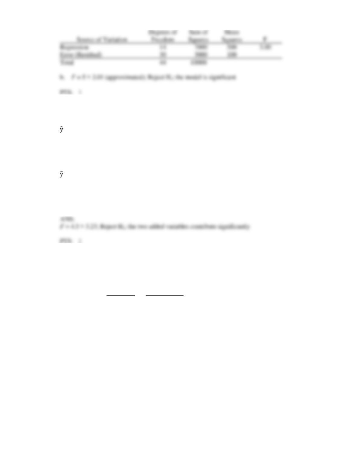
Fill in the blanks in the following ANOVA table.
b.
At = 0.05 level of significance, test to determine if the model is significant.
Source of Variation
Degrees of
Freedom
Sum of
Squares
Mean
Squares
F
Regression
_____?
_____?
_____?
_____?
Error (Residual)
_____?
_____?
_____?
Total
_____?
_____?
Degrees of
Sum of
Mean
Regression
42.12
Error (Residual)
Total
18. A regression analysis (involving 45 observations) relating a dependent variable (y) and two
independent variables resulted in the following information.
= 0.408 + 1.3387x1 + 2x2
The SSE for the above model is 49.
When two other independent variables were added to the model, the following information was
provided.
= 1.2 + 3.0x1 + 12x2 + 4.0x3 + 8x4
This latter model’s SSE is 40.
At a 5% significance level, test to determine if the two added independent variables contribute
significantly to the model.
19. A soft drink manufacturer has developed a regression model relating sales (y in $10,000) with four
independent variables. The four independent variables are price per unit (x1, in dollars), competitor’s
price (x2, in dollars), advertising (x3, in $1000) and type of container used (x4; 1 = Cans and 0 =
Bottles). Part of the regression results are shown below. (Assume n = 25)
Coefficient
Standard Error
Constant
443.143
x1
-57.170
20.426
x2
27.681
19.991
x3
0.025
0.023
x4
-95.353
91.027
a.
If the manufacturer uses can containers and if his price is $1.25, his advertising expenditure is
$200,000, and his competitor’s price is $1.50, what is your estimate of his sales? (Give your
answer in dollars.)
b.
Test to see if there is a significant relationship between sales and unit price. Let = 0.05.
c.
Test to see if there is a significant relationship between sales and advertising. Let = 0.05.
d.
Is the type of container a significant variable? Let = 0.05 = 0.05.
e.
Test to see if there is a significant relationship between sales and competitor’s price. Let =
0.05.
ANS:
Regression
Error (Residual)
Total
10000
b.
20. Thirty four observations of a dependent variable (y), and two independent variables resulted in an SSE
of 300. When a third independent variable was added to the model, the SSE was reduced to 250. At a
5% level of significance, determine if the third independent variable contributes significantly to the
model.
21. Forty-eight observations of a dependent variable (y) and five independent variables resulted in an SSE
of 438. When two additional independent variables were added to the model, the SSE was reduced to
375. At a 5% level of significance, determine if the two additional independent variables contribute
significantly to the model.
22. A regression analysis was applied in order to determine the relationship between a dependent variable
and 4 independent variables. The following information was obtained from the regression analysis.
R Square = 0.60
SSR = 4,800
Total number of observations n = 35
a.
Fill in the blanks in the following ANOVA table.
b.
At = 0.05 level of significance, test to determine if the model is significant.
Source of Variation
Degrees of
Freedom
Sum of
Squares
Mean
Squares
F
Regression
_____?
_____?
_____?
_____?
Error (Residual)
_____?
_____?
_____?
Total
_____?
_____?
Squares
11.25
a.
$3,228,490
b.
c.
d.
23. Consider the following data.
yi
xi
2
1
3
4
5
6
8
7
10
8
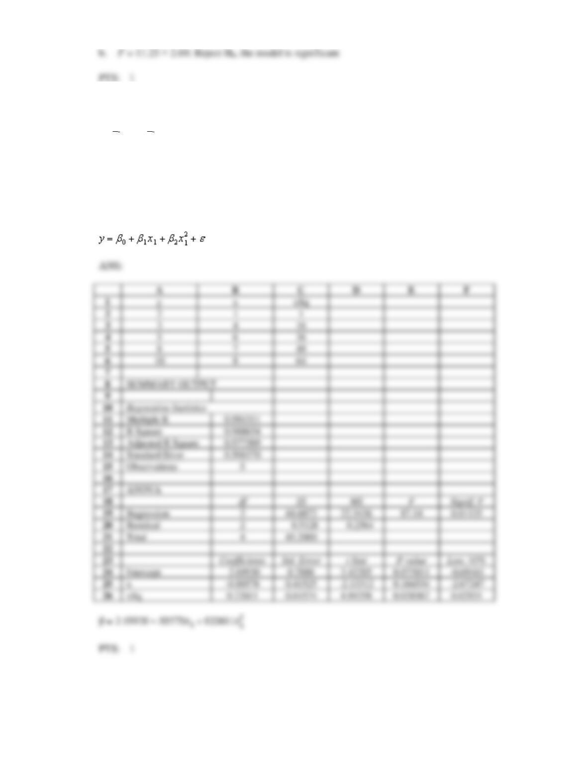
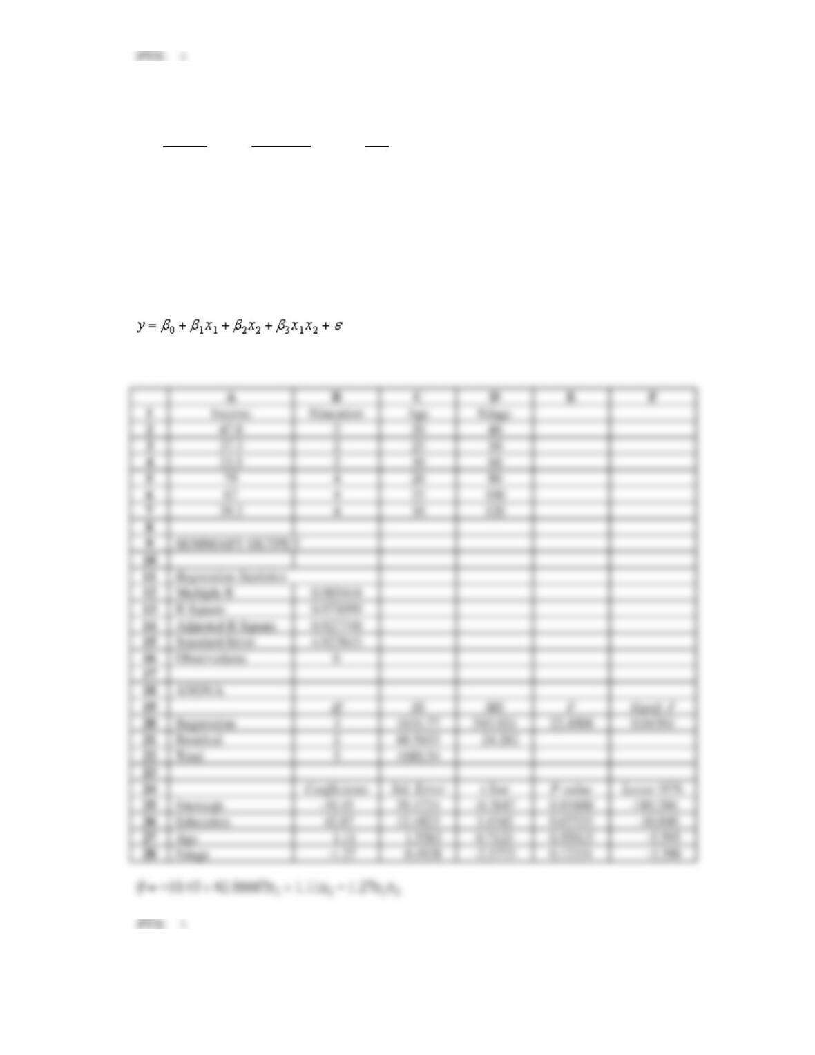
Use Excel’s Regression Tool to estimate a second-order model of the form
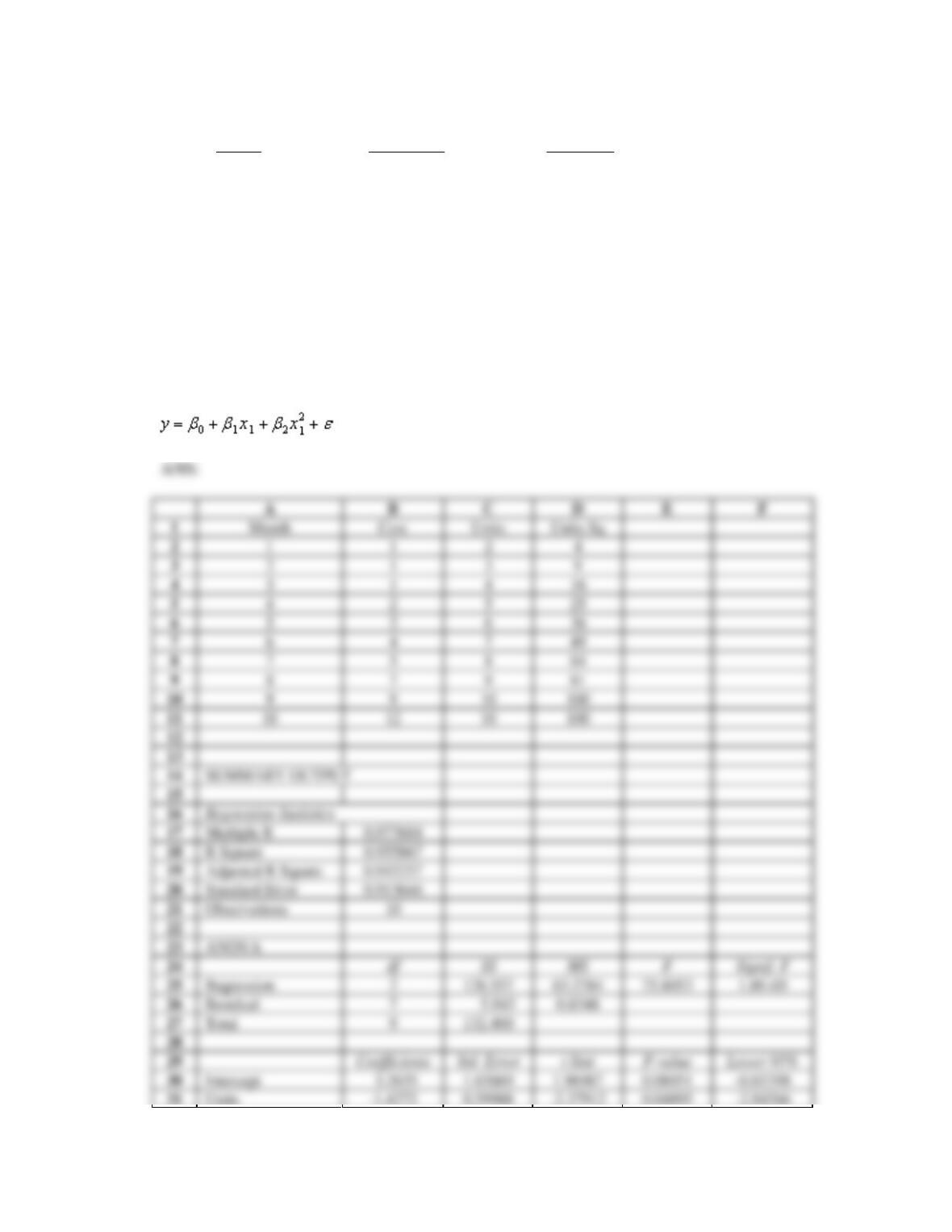
24. Monthly total production costs and the number of units produced at a local company over a period of
10 months are shown below.
Month
Production Costs (yi)
($millions)
Units Produced (xi)
(millions)
1
1
2
2
1
3
3
1
4
4
2
5
5
2
6
6
4
7
7
5
8
8
7
9
9
9
10
10
12
10
Use Excel’s Regression Tool to estimate a second-order model of the form
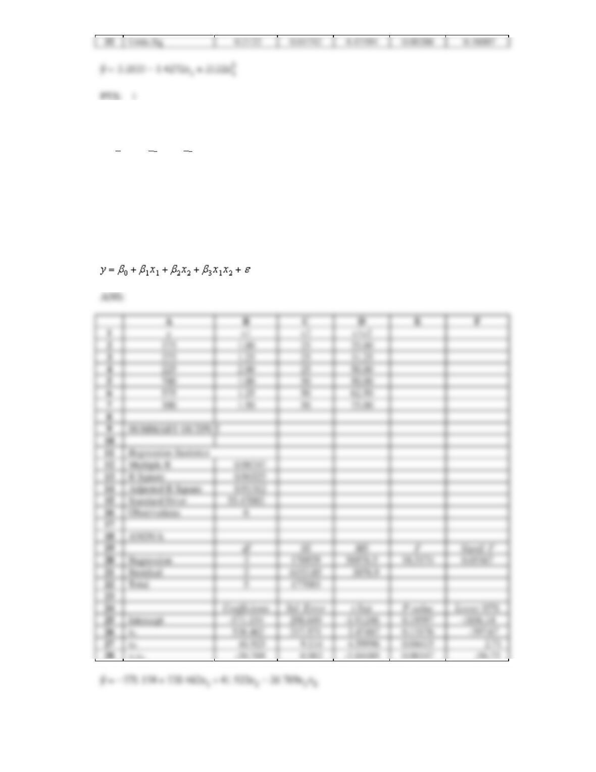
25. Consider the following data.
y
x1
x2
375
1.00
25
275
1.25
25
225
2.00
25
700
1.00
50
575
1.25
50
300
1.50
50
Use Excel’s Regression Tool to estimate a general linear model of the form
26. A sample of 6 recent college graduates shows their current annual income (in $1000), years of
education, and current age (in years). The data follow:
Income
Education
Age
47.8
2
20
37.3
2
25
33.5
2
30
79
4
20
67
4
25
39.3
4
30
Use Excel’s Regression Tool to estimate a general linear model of the form that predicts annual
income.
ANS:
27. Consider the following data.
y
x
2
1
3
4
5
6
8
7
10
8
Use Excel’s Regression Tool to estimate a general linear model of the form
ANS:
28. Consider the following data.
x
y
4
8
6
10
8
8
10
12
14
4
Use Excel’s Regression Tool to estimate a general linear model of the form
29. Consider the following data.
x
y
4
8
6
10
8
8
10
12
14
4
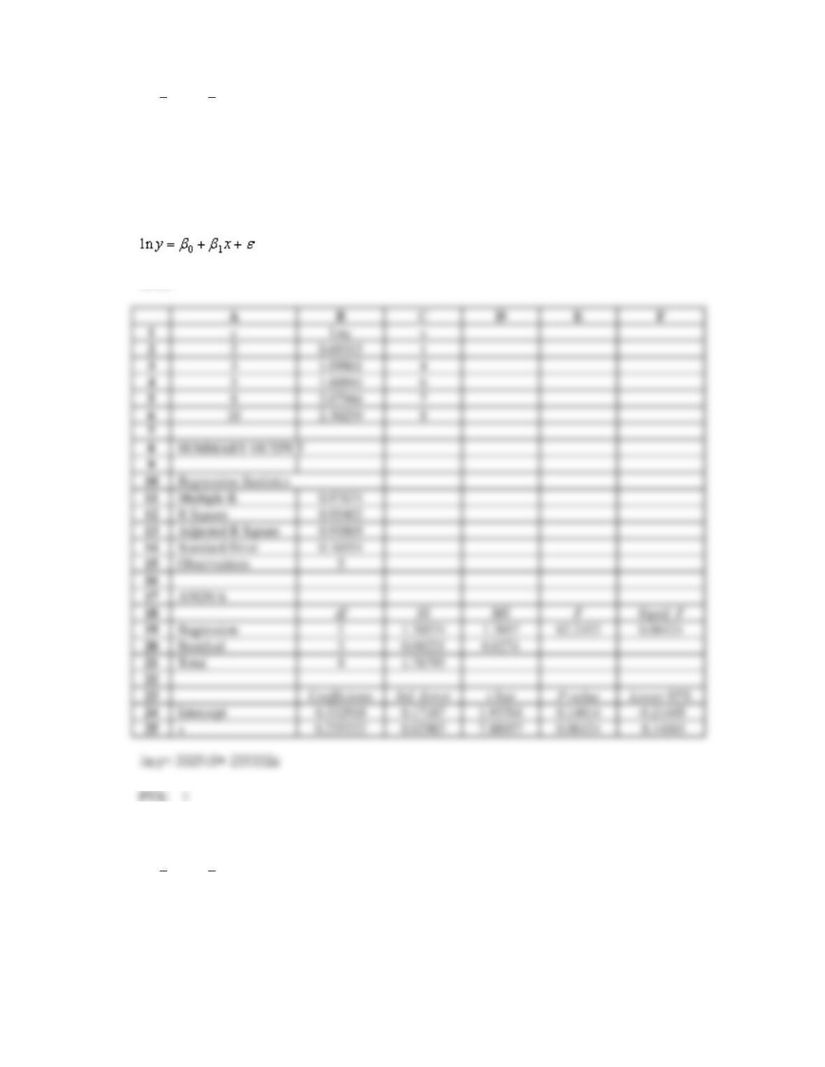
Use Excel’s Regression Tool to estimate a general linear model that uses a reciprocal transformation on
the dependent variable.
25
x
0.011712
0.00719
1.62852
0.20190
-0.01118
30. Consider the following data.
y
x
2
1
3
4
5
6
8
7
10
8
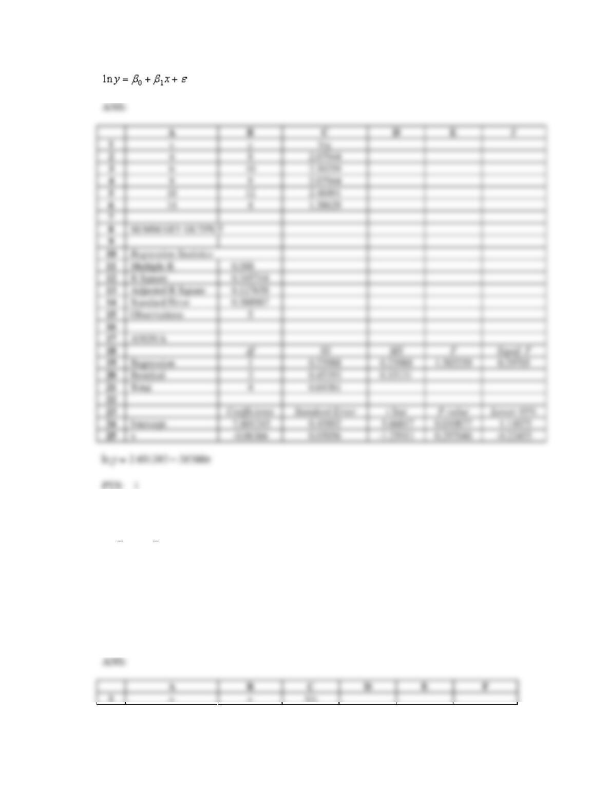
Use Excel’s Regression Tool to estimate a general linear model that uses a reciprocal transformation on
the dependent variable.
SUMMARY OUTPUT
SUMMARY OUTPUT
10
11
Multiple R
12
R Square
13
Adjusted R Square
14
Standard Error
15
Observations
16
17
18
19
Regression
0.00812
0.00812
2.65206
20
Residual
0.00919
0.00306
21
Total
0.01731
22
23
24
Intercept
0.038288
0.06528
0.58651
0.59875
-0.16947
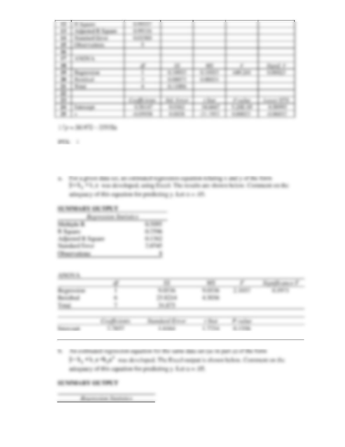
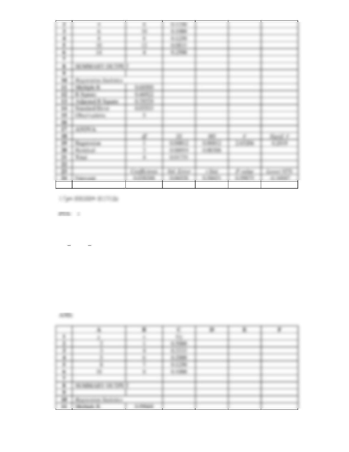
31. We are interested in determining what type of model best describes the relationship between two
variables x and y.
R Square
0.2596
Adjusted R Square
0.1362
Standard Error
2.0745
Observations
Regression
9.0536
9.0536
2.1037
Total
34.875
Intercept
2.7857
1.6164
1.7234
0.1356
x
0.4643
0.3201
1.4504
0.1971
Multiple R
0.9680
R Square
0.9370
Adjusted R Square
0.9118
Standard Error
0.6628
Observations
8
ANOVA
df
SS
MS
F
Significance F
Regression
2
32.6786
16.3392
37.1951
0.0010
Residual
5
2.1964
0.4393
Total
7
34.875
Coefficients
Standard Error
t Stat
P-value
Intercept
-2.8393
0.9247
-3.0706
0.0278
x
3.8393
0.4714
8.1437
0.0005
x-squared
-0.375
0.0511
-7.3335
0.0007
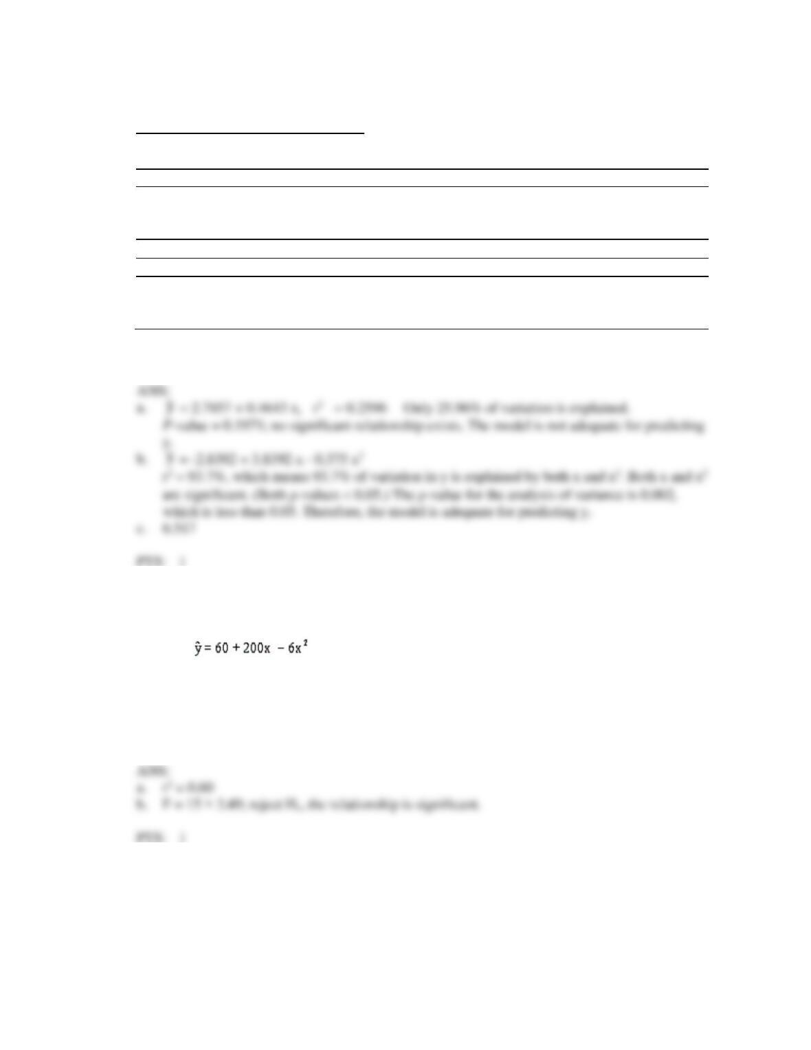
c.
Use the results of Part b and predict y when x = 4.
32. The following estimated regression equation has been developed for the relationship between y, the
dependent variable, and x, the independent variable.
The sample size for this regression model was 23, and SSR = 600 and SSE = 400.
a.
Compute the coefficient of determination.
b.
Using = .05, test for a significant relationship.
a.
b.
F = 15 > 3.49; reject Ho, the relationship is significant.
c.
6.517