
CHAPTER 16—REGRESSION ANALYSIS: MODEL BUILDING
MULTIPLE CHOICE
1. In multiple regression analysis, the general linear model
a.
cannot be used to accommodate curvilinear relationships between dependent variables and
independent variables
b.
can be used to accommodate curvilinear relationships between the independent variables
and dependent variable
c.
must contain more than 2 independent variables
d.
None of these alternatives is correct.
2. The following model
y = 0 + 1x1 +
is referred to as a
a.
curvilinear model
b.
curvilinear model with one predictor variable
c.
simple second-order model with one predictor variable
d.
simple first-order model with one predictor variable
3. In multiple regression analysis, the word “linear” in the term “general linear model” refers to the fact
that
a.
0, 1, . . . p, all have exponents of 0
b.
0, 1, . . . p, all have exponents of 1
c.
0, 1, . . . p, all have exponents of at least 1
d.
0, 1, . . . p, all have exponents of less than 1
4. Serial correlation is
a.
the correlation between serial numbers of products
b.
the same as autocorrelation
c.
the same as leverage
d.
None of these alternatives is correct.
5. The joint effect of two variables acting together is called
a.
autocorrelation
b.
interaction
c.
serial correlation
d.
joint regression
6. A test to determine whether or not first-order autocorrelation is present is
a.
a t test
b.
the Durbin-Watson test
c.
an F test
d.
a chi-square test
7. Which of the following tests is used to determine whether an additional variable makes a significant
contribution to a multiple regression model?
a.
a t test
b.
a Z test
c.
an F test
d.
a chi-square test
8. A variable such as z, whose value is z = x1x2 is added to a general linear model in order to account for
potential effects of two variables x1 and x2 acting together. This type of effect is
a.
impossible to occur
b.
called interaction
c.
called multicollinearity effect
d.
called transformation effect
9. The following regression model
y = 0 + 1x1 + 2x2 +
is known as
a.
first-order model with one predictor variable
b.
second-order model with two predictor variables
c.
second-order model with one predictor variable
d.
None of these alternatives is correct.
10. The parameters of nonlinear models have exponents
a.
larger than zero
b.
other than 1
c.
only equal to 2
d.
larger than 3
11. All the variables in a multiple regression analysis
a.
must be quantitative
b.
must be either quantitative or qualitative but not a mix of both
c.
must be positive
d.
None of these alternatives is correct.
12. The range of the Durbin-Watson statistic is between
a.
-1 to 1
b.
0 to 1
c.
-infinity to + infinity
d.
0 to 4

13. The correlation in error terms that arises when the error terms at successive points in time are related is
termed
a.
leverage
b.
multicorrelation
c.
autocorrelation
d.
parallel correlation
14. What value of Durbin-Watson statistic indicates no autocorrelation is present?
a.
1
b.
2
c.
-2
d.
0
Exhibit 16-1
In a regression analysis involving 25 observations, the following estimated regression equation was
developed.
= 10 – 18x1 + 3x2 + 14x3
Also, the following standard errors and the sum of squares were obtained.
Sb1 = 3 Sb2 = 6 Sb3 = 7
SST = 4,800 SSE = 1,296
15. Refer to Exhibit 16-1. If you want to determine whether or not the coefficients of the independent
variables are significant, the critical value of t statistic at = 0.05 is
a.
2.080
b.
2.060
c.
2.064
d.
1.96
16. Refer to Exhibit 16-1. The coefficient of x1
a.
is significant
b.
is not significant
c.
cannot be tested, because not enough information is provided
d.
None of these alternatives is correct.
17. Refer to Exhibit 16-1. The coefficient of x2
a.
is significant
b.
is not significant
c.
cannot be tested, because not enough information is provided
d.
None of these alternatives is correct.

18. Refer to Exhibit 16-1. The coefficient of x3
a.
is significant
b.
is not significant
c.
cannot be tested, because not enough information is provided
d.
None of these alternatives is correct.
19. Refer to Exhibit 16-1. The multiple coefficient of determination is
a.
0.27
b.
0.73
c.
0.50
d.
0.33
20. Refer to Exhibit 16-1. If we are interested in testing for the significance of the relationship among the
variables (i.e., significance of the model) the critical value of F at = 0.05 is
a.
2.76
b.
2.78
c.
3.10
d.
3.07
21. Refer to Exhibit 16-1. The test statistic for testing the significance of the model is
a.
0.730
b.
18.926
c.
3.703
d.
1.369
22. Refer to Exhibit 16-1. The model
a.
is significant
b.
is not significant
c.
may or may not be significant
d.
None of these alternatives is correct.
23. When dealing with the problem of non-constant variance, the reciprocal transformation means using
a.
1/x as the independent variable instead of x
b.
x2 as the independent variable instead of x
c.
y2 as the dependent variable instead of y
d.
1/y as the dependent variable instead of y
Exhibit 16-2
In a regression model involving 30 observations, the following estimated regression equation was
obtained.
= 170 + 34x1 – 3x2 + 8x3 + 58x4 + 3x5
24. Refer to Exhibit 16-2. The value of SSE is
a.
3,740
b.
170
c.
260
d.
2000
25. Refer to Exhibit 16-2. The degrees of freedom associated with SSR are
a.
24
b.
6
c.
19
d.
5
26. Refer to Exhibit 16-2. The degrees of freedom associated with SSE are
a.
24
b.
6
c.
19
d.
5
27. Refer to Exhibit 16-2. The degrees of freedom associated with SST are
a.
24
b.
6
c.
19
d.
None of these alternatives is correct.
28. Refer to Exhibit 16-2. The value of MSR is
a.
10.40
b.
348
c.
10.83
d.
52
29. Refer to Exhibit 16-2. The value of MSE is
a.
348
b.
10.40
c.
10.83
d.
32.13
30. Refer to Exhibit 16-2. The computed F value for testing the significance of the above model is
a.
32.12
b.
6.69
c.
4.8
d.
58

31. Refer to Exhibit 16-2. The coefficient of determination for this model is
a.
0.6923
b.
0.1494
c.
0.1300
d.
0.8700
Exhibit 16-3
Below you are given a partial Excel output based on a sample of 25 observations.
Coefficients
Standard Error
Intercept
145
29
x1
20
5
x2
-18
6
x3
4
4
32. Refer to Exhibit 16-3. The estimated regression equation is
a.
y = 0 + 1x1 + 2x2 + 3x3 +
b.
E(y) = 0 + 1x1 + 2x2 + 3x3
c.
= 29 + 5x1 + 6x2 + 4x3
d.
= 145 + 20x1 – 18x2 + 4x3
e.
None of the above answers are correct.
33. Refer to Exhibit 16-3. We want to test whether the parameter 2 is significant. The test statistic equals
a.
4
b.
5
c.
3
d.
-3
34. Refer to Exhibit 16-3. The critical t value obtained from the table to test an individual parameter at the
5% level is
a.
2.06
b.
2.069
c.
2.074
d.
2.080
Exhibit 16-4
In a laboratory experiment, data were gathered on the life span (y in months) of 33 rats, units of daily
protein intake (x1), and whether or not agent x2 (a proposed life extending agent) was added to the rats
diet (x2 = 0 if agent x2 was not added, and x2 = 1 if agent was added.) From the results of the
experiment, the following regression model was developed.
= 36 + 0.8x1 – 1.7x2
Also provided are SSR = 60 and SST = 180.

35. Refer to Exhibit 16-4. From the above function, it can be said that the life expectancy of rats that were
given agent x2 is
a.
1.7 months more than those who did not take agent x2
b.
1.7 months less than those who did not take agent x2
c.
0.8 months less than those who did not take agent x2
d.
0.8 months more than those who did not take agent x2
36. Refer to Exhibit 16-4. The life expectancy of a rat that was given 3 units of protein daily, and who
took agent x2 is
a.
36.7
b.
36
c.
49
d.
38.4
37. Refer to Exhibit 16-4. The life expectancy of a rat that was not given any protein and that did not take
agent x2 is
a.
36.7
b.
34.3
c.
36
d.
38.4
38. Refer to Exhibit 16-4. The degrees of freedom associated with SSR are
a.
3
b.
33
c.
32
d.
30
39. Refer to Exhibit 16-4. The degrees of freedom associated with SSE are
a.
3
b.
33
c.
32
d.
30
40. Refer to Exhibit 16-4. The multiple coefficient of determination is
a.
0.2
b.
0.5
c.
0.333
d.
5
41. Refer to Exhibit 16-4. If we want to test for the significance of the model, the critical value of F at
95% confidence is
a.
8.62
b.
3.35

c.
2.92
d.
2.96
42. Refer to Exhibit 16-4. The test statistic for testing the significance of the model is
a.
0.50
b.
5.00
c.
0.25
d.
0.33
43. Refer to Exhibit 16-4. The model
a.
is significant
b.
is not significant
c.
Not enough information is provided to answer this question.
d.
None of these alternatives is correct.
44. Refer to Exhibit 16-4. The life expectancy of a rat that was given 2 units of agent x2 daily, but was not
given any protein is
a.
32.6
b.
36
c.
38
d.
34.3
45. Excel’s Regression tool can be used to perform the ____ procedure.
a.
stepwise regression
b.
forward selection
c.
backward elimination
d.
best-subsets
46. The forward selection procedure starts with how many independent variable(s) in the multiple
regression model?
a.
none
b.
one
c.
two
d.
all of them
47. Which of the following statements about the backward elimination procedure is false?
a.
It is a one-variable-at-a-time procedure.
b.
It begins with the regression model found using the forward selection procedure.
c.
It does not permit an independent variable to be reentered once it has been removed.
d.
It does not guarantee that the best regression model will be found.
48. The null hypothesis in the Durbin-Watson test is always that there is

a.
positive autocorrelation
b.
negative autocorrelation
c.
either positive or negative autocorrelation
d.
no autocorrelation
49. When autocorrelation is present, one of the assumptions of the regression model is violated and that
assumption is:
a.
the expected value of the error term
is zero
b.
the variance of the error term
is the same for all values of x
c.
the values of the error term
are independent
d.
the values of the error term
are normally distributed for all values of x
50. The variable selection procedure that identifies the best regression equation, given a specified number
of independent variables, is
a.
stepwise regression
b.
forward selection
c.
backward elimination
d.
best-subsets regression
PROBLEM
1. Monthly total production costs and the number of units produced at a local company over a period of
10 months are shown below.
Month
Production Costs (yi)
($millions)
Units Produced (xi)
(millions)
1
1
2
2
1
3
3
1
4
4
2
5
5
2
6
6
4
7
7
5
8
8
7
9
9
9
10
10
12
10
a.
Draw a scatter diagram for the above data.
b.
Assume that a model in the form of
y = 0 + 1 +
best describes the relationship between x and y. Estimate the parameters of this curvilinear
regression equation.
2. Consider the following data.
yi
xi
2
1
3
4
5
6
8
7
10
8
a.
Draw a scatter diagram. Does the relationship between x and y appear to be linear?
b.
Assume the relationship between x and y can best be given by
y = 0 + 1 +
Estimate the parameters of this curvilinear function.
a.
Relationship appears to be curvilinear
3. Part of an Excel output relating y (dependent variable) and 4 independent variables, x1 through x4, is
shown below.
Summary Output
Regression Statistics
Multiple R
?
R Square
?
Adjusted R Square
?
Standard Error
72.6093
Observations
20
ANOVA
df
SS
MS
F
Significance F
Regression
?
422975.2376
?
?
0.0000
Residual
?
?
?
Total
?
?
Coefficients
Standard Error
t Stat
P-value
Intercept
-203.6125
100.2940
?
0.0605
x1
0.6483
0.1110
?
0.0000
x2
0.0190
0.0065
?
0.0101
x3
40.4577
7.5940
?
0.0001
x4
-0.1032
20.7823
?
0.9961
a.
Fill in all the blanks marked with “?”
b.
At a 5% significance level, which independent variables are significant and which ones are
not? Fully explain how you arrived at your answers.
Summary Output
b.
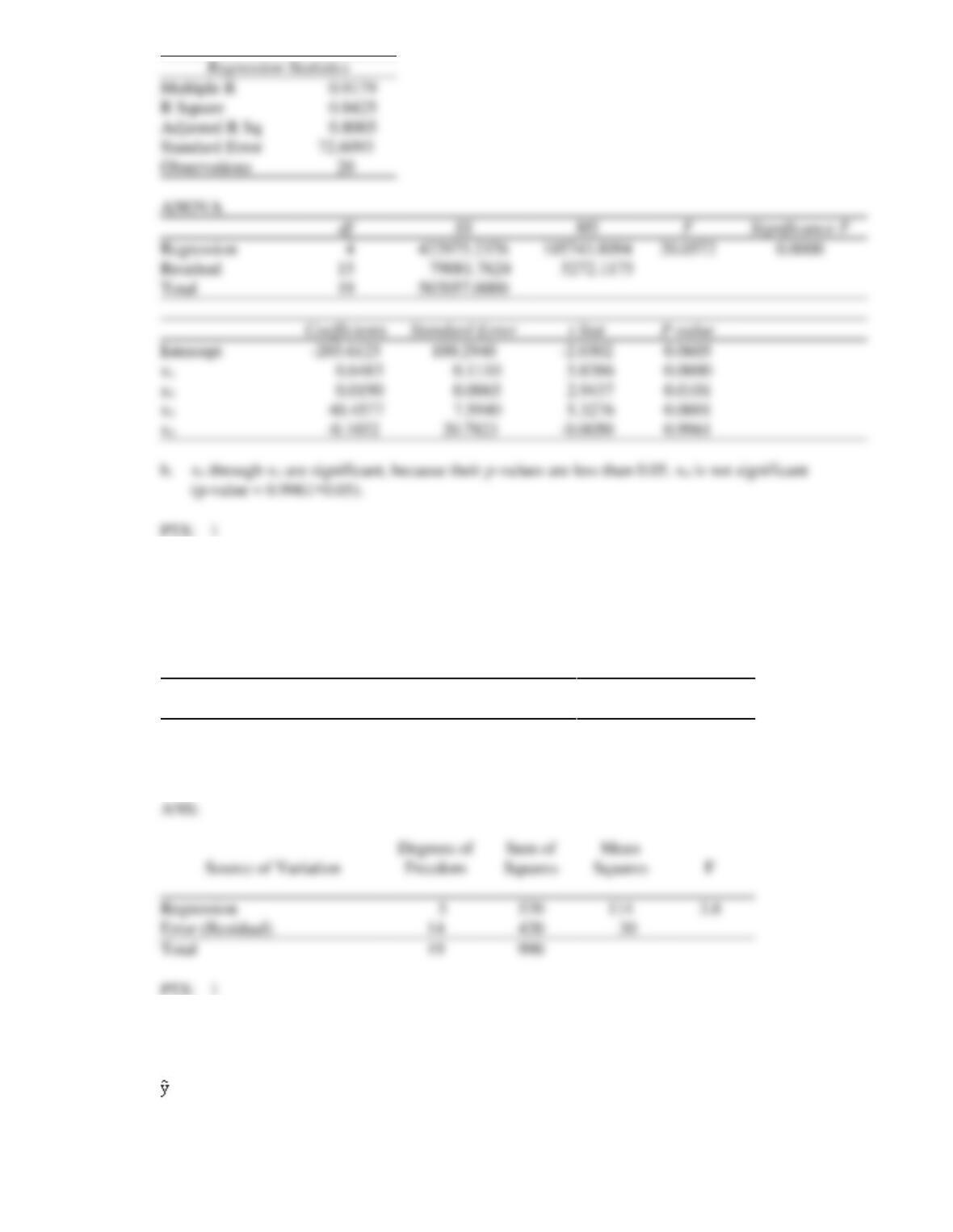
4. In a regression analysis involving 20 observations and five independent variables, the following
information was obtained.
Source of Variation
Degrees of
Freedom
Sum of
Squares
Mean
Squares
F
Regression
_____?
_____?
_____?
_____?
Error (Residual)
_____?
_____?
30
Total
_____?
990
Fill in all the blanks in the above ANOVA table.
Source of Variation
Freedom
Regression
Error (Residual)
Total
5. A researcher is trying to decide whether or not to add another variable to his model. He has estimated
the following model from a sample of 28 observations.
= 23.62 + 18.86x1 + 24.72x2
Multiple R
R Square
Adjusted R Sq
Standard Error
Observations
Regression
Residual
Total
Intercept
SSE = 1,425 SSR = 1,326
He has also estimated the model with an additional variable x3. The results are
= 25.32 + 15.29x1 + 7.63x2 + 12.72x3
SSE = 1,300 SSR = 1,451
What advice would you give this researcher? Use a .05 level of significance.
6. We want to test whether or not the addition of 3 variables to a model will be statistically significant.
You are given the following information based on a sample of 25 observations.
= 62.42 – 1.836x1 + 25.62x2
SSE = 725 SSR = 526
The equation was also estimated including the 3 variables. The results are
= 59.23 – 1.762x1 + 25.638x2 + 16.237x3 + 15.297x4 – 18.723x5
SSE = 520 SSR = 731
a.
State the null and alternative hypotheses.
b.
Test the null hypothesis at the 5% level of significance.
Ha: at least one of the coefficients is not equal to zero
b.
Do not reject H0; 2.497 < 3.13
7. Multiple regression analysis was used to study the relationship between a dependent variable, y, and
three independent variables x1, x2 and, x3. The following is a partial result of the regression analysis
involving 20 observations.
ANALYSIS OF VARIANCE
Source of Variation
Degrees of
Freedom
Sum of
Squares
Mean
Squares
F
Regression
80
Error
320
Coefficient
Standard Error
Constant
20.00
5.00
x1
15.00
3.00
x2
8.00
5.00
x3
-18.00
10.00
a.
Compute the coefficient of determination.
b.
Perform a t test and determine whether or not 1 is significantly different from zero ( = 0.05).
c.
Perform a t test and determine whether or not 2 is significantly different from zero ( = 0.05).
d.
Perform a t test and determine whether or not 3 is significantly different from zero ( = 0.05).
e.
At = 0.05, perform an F test and determine whether or not the regression model is significant.
8. Multiple regression analysis was used to study the relationship between a dependent variable, y, and
four independent variables; x1, x2, x3 and, x4. The following is a partial result of the regression analysis
involving 31 observations.
ANALYSIS OF VARIANCE
Source of
Variation
Degrees of
Freedom
Sum of
Squares
Mean
Squares
F
Regression
125
Error
Total
760
Coefficient
Standard Error
Constant
18.00
6.00
x1
12.00
8.00
x2
24.00
48.00
x3
-36.00
36.00
x4
16.00
2.00
a.
Compute the coefficient of determination.
b.
At = 0.05, perform an F test and determine whether or not the regression model is
significant.
c.
Perform a t test and determine whether or not 1 is significantly different from zero ( = 0.05).
d.
Perform a t test and determine whether or not 4 is significantly different from zero ( = 0.05).
a.
0.6579
b.
c.
d.
a.
0.3636
b.
d.