Simple Linear Regression 13-1
CHAPTER 13: SIMPLE LINEAR REGRESSION
1. The Y-intercept (b0) represents the
a) predicted value of Y when X = 0.
b) change in estimated Y per unit change in X.
c) predicted value of Y.
d) variation around the sample regression line.
2. The Y-intercept (b0) represents the
a) estimated average Y when X = 0.
b) change in estimated average Y per unit change in X.
c) predicted value of Y.
d) variation around the sample regression line.
3. The slope (b1) represents
a) predicted value of Y when X = 0.
b) the estimated average change in Y per unit change in X.
c) the predicted value of Y.
d) variation around the line of regression.
4. The least squares method minimizes which of the following?
a) SSR
b) SSE
c) SST
d) All of the above
13-2 Simple Linear Regression
SCENARIO 13-1
A large national bank charges local companies for using their services. A bank official reported the
results of a regression analysis designed to predict the bank’s charges (Y) — measured in dollars per
month — for services rendered to local companies. One independent variable used to predict service
charges to a company is the company’s sales revenue (X) — measured in millions of dollars. Data for
21 companies who use the bank’s services were used to fit the model:
01iii
YX
ββ
ε
=+ +
The results of the simple linear regression are provided below.
l
2,700 20 , 65, two-tail value 0.034 (for testing )
YX
YXS p
β
1
=− + = =
5. Referring to Scenario 13-1, interpret the estimate of
β
0, the Y-intercept of the line.
a) All companies will be charged at least $2,700 by the bank.
b) There is no practical interpretation since a sales revenue of $0 is a nonsensical value.
c) About 95% of the observed service charges fall within $2,700 of the least squares line.
d) For every $1 million increase in sales revenue, we expect a service charge to decrease
$2,700.
6. Referring to Scenario 13-1, interpret the estimate of
σ
, the standard deviation of the random
error term (standard error of the estimate) in the model.
a) About 95% of the observed service charges fall within $65 of the least squares line.
b) About 95% of the observed service charges equal their corresponding predicted values.
c) About 95% of the observed service charges fall within $130 of the least squares line.
d) For every $1 million increase in sales revenue, we expect a service charge to increase
$65.
7. Referring to Scenario 13-1, interpret the p-value for testing whether
β
1 exceeds 0.
a) There is sufficient evidence (at the
α
= 0.05) to conclude that sales revenue (X) is a
useful linear predictor of service charge (Y).
b) There is insufficient evidence (at the
α
= 0.10) to conclude that sales revenue (X) is a
useful linear predictor of service charge (Y).
c) Sales revenue (X) is a poor predictor of service charge (Y).
d) For every $1 million increase in sales revenue, you expect a service charge to increase
$0.034.
Simple Linear Regression 13-3
8. Referring to Scenario 13-1, a 95% confidence interval for
β
1 is (15, 30). Interpret the interval.
a) You are 95% confident that the mean service charge will fall between $15 and $30 per
month.
b) You are 95% confident that the sales revenue (X) will increase between $15 and $30
million for every $1 increase in service charge (Y).
c) You are 95% confident that mean service charge (Y) will increase between $15 and $30
for every $1 million increase in sales revenue (X).
d) At the
α
= 0.05 level, there is no evidence of a linear relationship between service
charge (Y) and sales revenue (X).
SCENARIO 13-2
A candy bar manufacturer is interested in trying to estimate how sales are influenced by the price of
their product. To do this, the company randomly chooses 6 small cities and offers the candy bar at
different prices. Using candy bar sales as the dependent variable, the company will conduct a simple
linear regression on the data below:
City Price ($) Sales
River Falls 1.30 100
Hudson 1.60 90
Ellsworth 1.80 90
Prescott 2.00 40
Rock Elm 2.40 38
Stillwater 2.90 32
9. Referring to Scenario 13-2, what is the estimated slope for the candy bar price and sales data?
a) 161.386
b) 0.784
c) – 3.810
d) – 48.193
13-4 Simple Linear Regression
10. Referring to Scenario 13-2, what is the estimated mean change in the sales of the candy bar if
price goes up by $1.00?
a) 161.386
b) 0.784
c) – 3.810
d) – 48.193
11. Referring to Scenario 13-2, what is the coefficient of correlation for these data?
a) – 0.8854
b) – 0.7839
c) 0.7839
d) 0.8854
12. Referring to Scenario 13-2, what is the percentage of the total variation in candy bar sales
explained by the regression model?
a) 100%
b) 88.54%
c) 78.39%
d) 48.19%
13. Referring to Scenario 13-2, what percentage of the total variation in candy bar sales is explained
by prices?
a) 100%
b) 88.54%
c) 78.39%
d) 48.19%
Simple Linear Regression 13-5
14. Referring to Scenario 13-2, what is the standard error of the estimate, SYX, for the data?
a) 0.784
b) 0.885
c) 12.650
d) 16.299
15. Referring to Scenario 13-2, what is the standard error of the regression slope estimate, 1
b
S?
a) 0.784
b) 0.885
c) 12.650
d) 16.299
16. Referring to Scenario 13-2, what is
∑
(X–X )2 for these data?
a) 0
b) 1.66
c) 2.54
d) 25.66
17. Referring to Scenario 13-2, to test that the regression coefficient,
β
1, is not equal to 0, what
would be the critical values? Use
α
= 0.05.
a) ± 2.5706
b) ± 2.7764
c) ± 3.1634
d) ± 3.4954
13-6 Simple Linear Regression
18. Referring to Scenario 13-2, to test whether a change in price will have any impact on sales, what
would be the critical values? Use
α
= 0.05.
a) ± 2.5706
b) ± 2.7765
c) ± 3.1634
d) ± 3.4954
19. Referring to Scenario 13-2, if the price of the candy bar is set at $2, the estimated mean sales will
be
a) 30
b) 65
c) 90
d) 100
20. Referring to Scenario 13-2, if the price of the candy bar is set at $2, the predicted sales will be
a) 30
b) 65
c) 90
d) 100
21. True of False: The Chancellor of a university has commissioned a team to collect data on
students’ GPAs and the amount of time they spend bar hopping every week (measured in
minutes). He wants to know if imposing much tougher regulations on all campus bars to make it
more difficult for students to spend time in any campus bar will have a significant impact on
general students’ GPAs. His team should use a t test on the slope of the population regression.
Simple Linear Regression 13-7
22. The residual represents the discrepancy between the observed dependent variable and its
_______ value.
SCENARIO 13-3
The director of cooperative education at a state college wants to examine the effect of cooperative
education job experience on marketability in the work place. She takes a random sample of 4
students. For these 4, she finds out how many times each had a cooperative education job and how
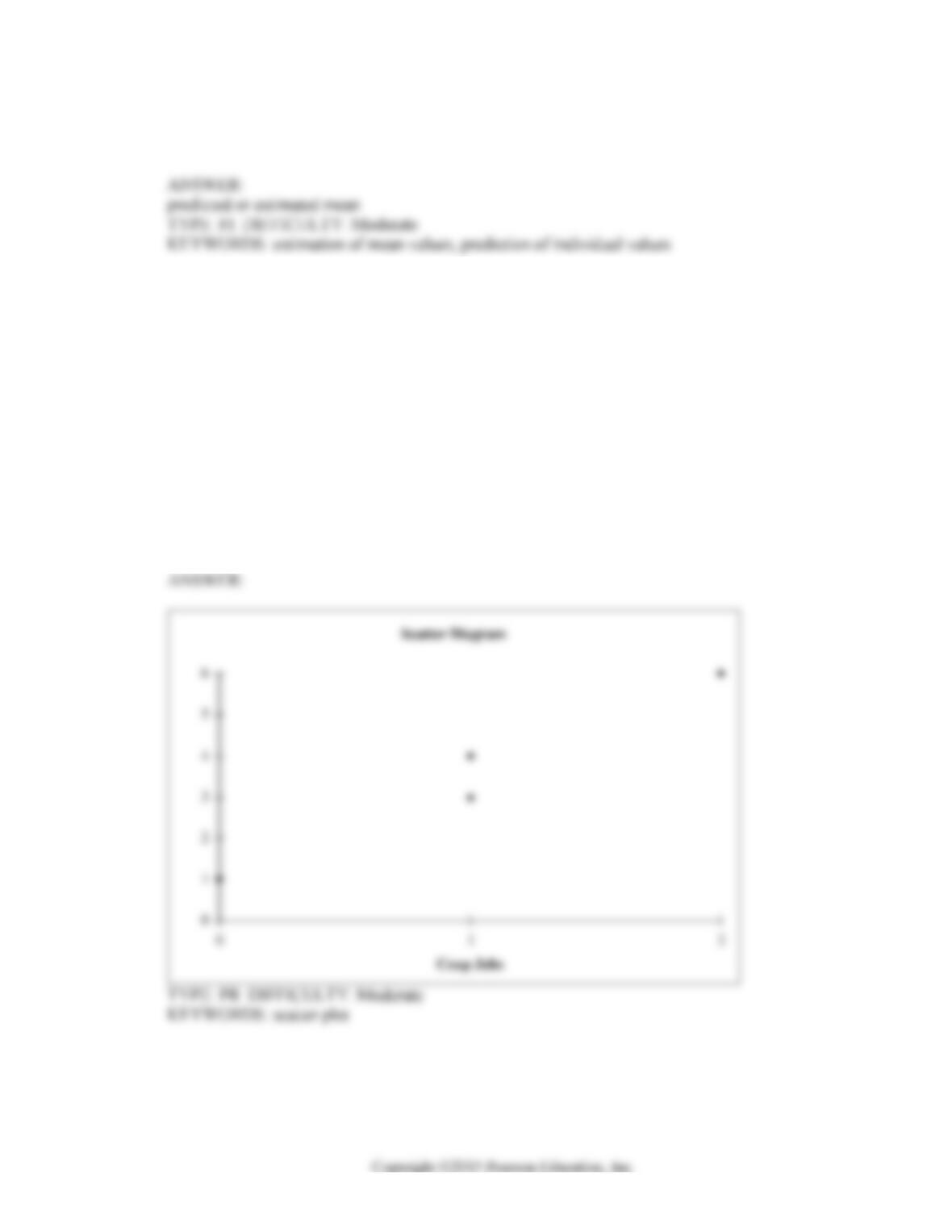
many job offers they received upon graduation. These data are presented in the table below.
Student CoopJobs JobOffer
1 1 4
2 2 6
3 1 3
4 0 1
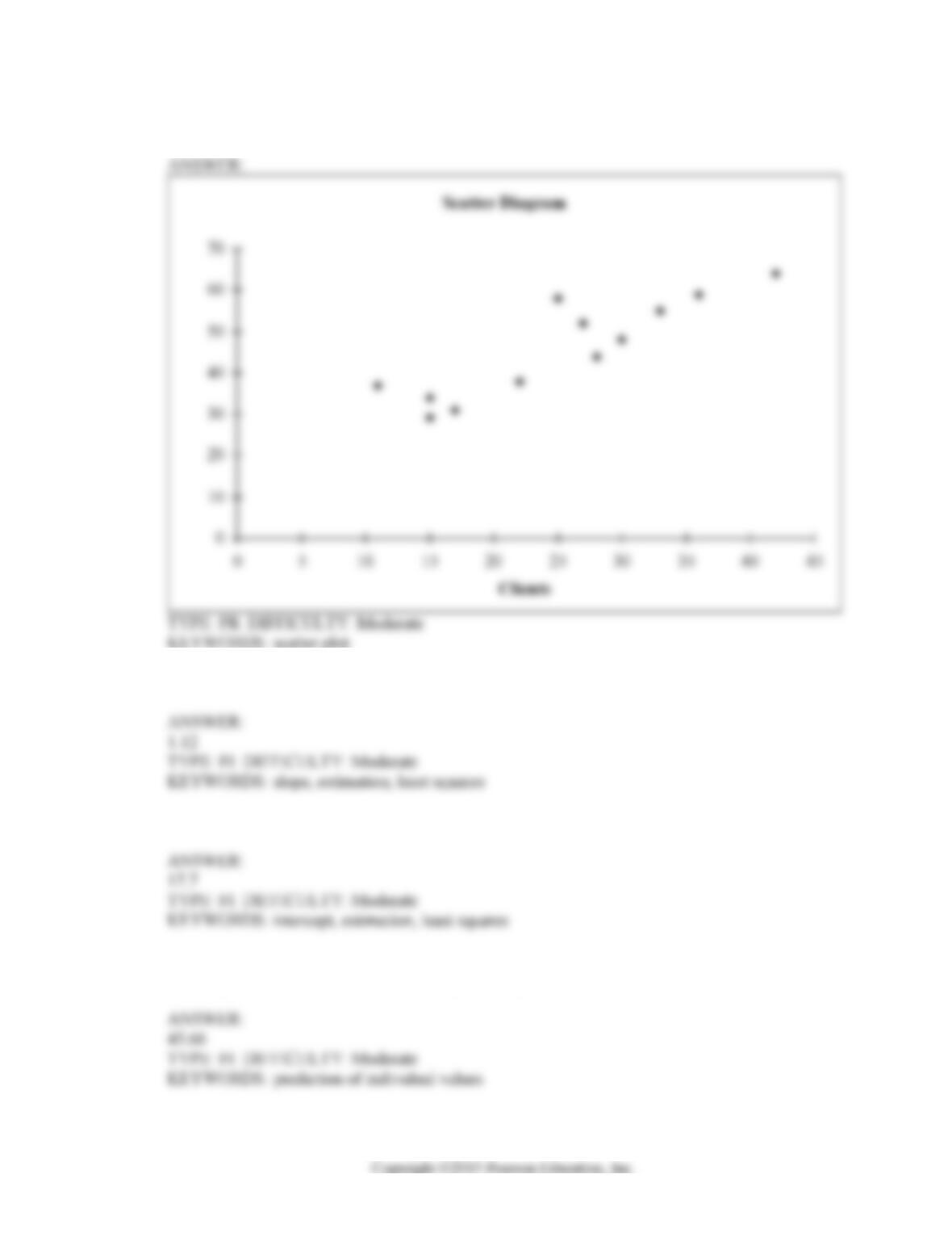
23. Referring to Scenario 13-3, set up a scatter plot.
13-8 Simple Linear Regression
24. Referring to Scenario 13-3, the least squares estimate of the slope is __________.
25. Referring to Scenario 13-3, the least squares estimate of the Y-intercept is __________.
26. Referring to Scenario 13-3, the prediction for the number of job offers for a person with 2 coop
jobs is __________.
27. Referring to Scenario 13-3, the total sum of squares (SST) is __________.
28. Referring to Scenario 13-3, the regression sum of squares (SSR) is __________.
29. Referring to Scenario 13-3, the error or residual sum of squares (SSE) is __________.
30. Referring to Scenario 13-3, the coefficient of determination is __________.
Simple Linear Regression 13-9
31. Referring to Scenario 13-3, the standard error of estimate is __________.
32. Referring to Scenario 13-3, the coefficient of correlation is __________.
33. Referring to Scenario 13-3, suppose the director of cooperative education wants to construct a
95% confidence-interval estimate for the mean number of job offers received by students who
have had exactly one cooperative education job. The t critical value she would use is ________.
34. Referring to Scenario 13-3, suppose the director of cooperative education wants to construct a
95% confidence interval estimate for the mean number of job offers received by students who
have had exactly one cooperative education job. The confidence interval is from ________ to
________.
35. Referring to Scenario 13-3, suppose the director of cooperative education wants to construct a
95% prediction interval estimate for the number of job offers received by students who have had
exactly one cooperative education job. The prediction interval is from ________ to ________.
13-10 Simple Linear Regression
36. True or False: Referring to Scenario 13-3, suppose the director of cooperative education wants to
construct two 95% confidence interval estimates. One is for the mean number of job offers
received by students who have had exactly one cooperative education job and one for students
who have had two. The confidence interval for students who have had one cooperative education
job would be the wider of the two intervals.
37. Referring to Scenario 13-3, suppose the director of cooperative education wants to construct a
95% prediction interval for the number of job offers received by a student who has had exactly
two cooperative education jobs. The t critical value she would use is ________.
38. Referring to Scenario 13-3, suppose the director of cooperative education wants to construct a
95% prediction interval for the number of job offers received by a student who has had exactly
two cooperative education jobs. The prediction interval is from ________ to ________.
39. True or False: Referring to Scenario 13-3, suppose the director of cooperative education wants to
construct both a 95% confidence interval estimate and a 95% prediction interval for X = 2. The
confidence interval estimate would be the wider of the two intervals.
40. Referring to Scenario 13-3, the director of cooperative education wanted to test the hypothesis
that the population slope was equal to 0. The denominator of the test statistic is
s
b1. The value of
s
b1 in this sample is ________.
Simple Linear Regression 13-11
41. Referring to Scenario 13-3, the director of cooperative education wanted to test the hypothesis
that the population slope was equal to 0. The value of the test statistic is ________.
42. Referring to Scenario 13-3, the director of cooperative education wanted to test the hypothesis
that the population slope was equal to 3.0. The value of the test statistic is ________.
43. Referring to Scenario 13-3, the director of cooperative education wanted to test the hypothesis
that the population slope was equal to 0. For a test with a level of significance of 0.05, the null
hypothesis should be rejected if the value of the test statistic is ________.
44. Referring to Scenario 13-3, the director of cooperative education wanted to test the hypothesis
that the population slope was equal to 3.0. For a test with a level of significance of 0.05, the null
hypothesis should be rejected if the value of the test statistic is ________.
45. Referring to Scenario 13-3, the director of cooperative education wanted to test the hypothesis
that the population slope was equal to 0. The p-value of the test is between ________ and
________.
13-12 Simple Linear Regression
46. Referring to Scenario 13-3, the director of cooperative education wanted to test the hypothesis
that the population slope was equal to 3.0. The p-value of the test is between ________ and
________.
EXPLANATION: The t-test statistic is
()()
1
11 2.5 3 1.4142
0.3536
b
b
tS
β
−−
===−
KEYWORDS: t test on slope, p-value, slope
SCENARIO 13-4
The managers of a brokerage firm are interested in finding out if the number of new clients a broker
brings into the firm affects the sales generated by the broker. They sample 12 brokers and determine
the number of new clients they have enrolled in the last year and their sales amounts in thousands of
dollars. These data are presented in the table that follows.
Broker Clients Sales
1 27 52
2 11 37
3 42 64
4 33 55
5 15 29
6 15 34
7 25 58
8 36 59
9 28 44
10 30 48
11 17 31
12 22 38
Simple Linear Regression 13-13
47. Referring to Scenario 13-4, set up a scatter plot.
48. Referring to Scenario 13-4, the least squares estimate of the slope is __________.
49. Referring to Scenario 13-4, the least squares estimate of the Y-intercept is __________.
50. Referring to Scenario 13-4, the prediction for the amount of sales (in $1,000s) for a person who
brings 25 new clients into the firm is ________.
13-14 Simple Linear Regression
51. Referring to Scenario 13-4, the total sum of squares (SST) is __________.
52. Referring to Scenario 13-4, the regression sum of squares (SSR) is __________.
53. Referring to Scenario 13-4, the error or residual sum of squares (SSE) is __________.
54. Referring to Scenario 13-4, the coefficient of determination is __________.
55. Referring to Scenario 13-4, ______% of the total variation in sales generated can be explained by
the number of new clients brought in.
56. Referring to Scenario 13-4, the standard error of the estimated slope coefficient is __________.
57. Referring to Scenario 13-4, the standard error of estimate is __________.
Simple Linear Regression 13-15
58. Referring to Scenario 13-4, the coefficient of correlation is __________.
59. Referring to Scenario 13-4, suppose the managers of the brokerage firm want to construct a 99%
confidence interval estimate for the mean sales made by brokers who have brought into the firm
24 new clients. The t critical value they would use is ________.
60. Referring to Scenario 13-4, suppose the managers of the brokerage firm want to construct a 99%
confidence interval estimate for the mean sales made by brokers who have brought into the firm
24 new clients. The confidence interval is from ________ to ________.
61. Referring to Scenario 13-4, suppose the managers of the brokerage firm want to construct n a
99% prediction interval for the sales made by a broker who has brought into the firm 18 new
clients. The t critical value they would use is ________.
62. Referring to Scenario 13-4, suppose the managers of the brokerage firm want to construct a 99%
prediction interval for the sales made by a broker who has brought into the firm 18 new clients.
The prediction interval is from ________ to ________.
13-16 Simple Linear Regression
63. Referring to Scenario 13-4, suppose the managers of the brokerage firm want to construct both a
99% confidence interval estimate and a 99% prediction interval for X = 24. The confidence
interval estimate would be the __________ (wider or narrower) of the two intervals.
64. Referring to Scenario 13-4, the managers of the brokerage firm wanted to test the hypothesis that
the population slope was equal to 0. The denominator of the test statistic is
s
b1. The value of
s
b1
in this sample is ________.
65. Referring to Scenario 13-4, the managers of the brokerage firm wanted to test the hypothesis that
the population slope was equal to 0. The value of the test statistic is _______.
66. Referring to Scenario 13-4, the managers of the brokerage firm wanted to test the hypothesis that
the number of new clients brought in did not affect the amount of sales generated. The value of
the test statistic is _______.
67. Referring to Scenario 13-4, the managers of the brokerage firm wanted to test the hypothesis that
the population slope was equal to 0. For a test with a level of significance of 0.01, the null
hypothesis should be rejected if the value of the test statistic is ________.
Simple Linear Regression 13-17
68. Referring to Scenario 13-4, the managers of the brokerage firm wanted to test the hypothesis that
the population slope was equal to 0. The p-value of the test is ________.
69. Referring to Scenario 13-4, the managers of the brokerage firm wanted to test the hypothesis that
the population slope was equal to 0. At a level of significance of 0.01, the null hypothesis should
be _______ (rejected or not rejected).
70. Referring to Scenario 13-4, the managers of the brokerage firm wanted to test the hypothesis that
the population slope was equal to 0. At a level of significance of 0.01, the decision that should be
made implies that _____ (there is a or there is no) linear dependent relationship between the
independent and dependent variables.
71. Referring to Scenario 13-4, the managers of the brokerage firm wanted to test the hypothesis that
the number of new clients brought in had a positive impact on the amount of sales generated. The
value of the test statistic is _______.
72. Referring to Scenario 13-4, the managers of the brokerage firm wanted to test the hypothesis that
the number of new clients brought in had a positive impact on the amount of sales generated. For
a test with a level of significance of 0.01, the null hypothesis should be rejected if the value of the
test statistic is ________.
13-18 Simple Linear Regression
73. Referring to Scenario 13-4, the managers of the brokerage firm wanted to test the hypothesis that
the number of new clients brought in had a positive impact on the amount of sales generated. The
p-value of the test is ________.
74. Referring to Scenario 13-4, the managers of the brokerage firm wanted to test the hypothesis that
the number of new clients brought in had a positive impact on the amount of sales generated. At a
level of significance of 0.01, the null hypothesis should be _______ (rejected or not rejected).
75. Referring to Scenario 13-4, the managers of the brokerage firm wanted to test the hypothesis that
the number of new clients brought in had a positive impact on the amount of sales generated. At a
level of significance of 0.01, the decision that should be made implies that the number of new
clients brought in _____ (had or did not have) a positive impact on the amount of sales
generated.
Simple Linear Regression 13-19
SCENARIO 13-5
The managing partner of an advertising agency believes that his company’s sales are related to the
industry sales. He uses Microsoft Excel to analyze the last 4 years of quarterly data (i.e., n = 16) with
the following results:
Regression Statistics
Multiple R 0.802
R Square 0.643
Adjusted R Square 0.618
Standard Error SYX 0.9224
Observations 16
ANOVA
df SS MS F Sig.F
Regression 1 21.497 21.497 25.27 0.000
Error 14 11.912 0.851
Total 15 33.409
Predictor Coef StdError t Stat P-value
Intercept 3.962 1.440 2.75 0.016
Industry 0.040451 0.008048 5.03 0.000
Durbin-Watson Statistic 1.59
76. Referring to Scenario 13-5, the value of the quantity that the least squares regression line
minimizes is ________.
77. Referring to Scenario 13-5, the estimates of the Y-intercept and slope are ________ and
________, respectively.
78. Referring to Scenario 13-5, the prediction for a quarter in which X = 120 is Y = ________.
13-20 Simple Linear Regression
79. Referring to Scenario 13-5, the standard error of the estimate is ________.
80. Referring to Scenario 13-5, the coefficient of determination is ________.
81. Referring to Scenario 13-5, the standard error of the estimated slope coefficient is ________.
82. Referring to Scenario 13-5, the correlation coefficient is ________.
83. Referring to Scenario 13-5, the partner wants to test for autocorrelation using the Durbin-Watson
statistic. Using a level of significance of 0.05, the critical values of the test are dL = ________,
and dU = ________.
84. Referring to Scenario 13-5, the partner wants to test for autocorrelation using the Durbin-Watson
statistic. Using a level of significance of 0.05, the decision he should make is:
a) there is evidence of autocorrelation.
b) the test is unable to make a definite conclusion.
c) there is no evidence of autocorrelation.
d) there is not enough information to perform the test.
Simple Linear Regression 13-21
85. If the Durbin-Watson statistic has a value close to 0, which assumption is violated?
a) Normality of the errors.
b) Independence of errors.
c) Homoscedasticity.
d) None of the above.
86. If the Durbin-Watson statistic has a value close to 4, which assumption is violated?
a) Normality of the errors.
b) Independence of errors.
c) Homoscedasticity.
d) None of the above.
87. The standard error of the estimate is a measure of
a) total variation of the Y variable.
b) the variation around the sample regression line.
c) explained variation.
d) the variation of the X variable.
88. The coefficient of determination (r2) tells you
a) that the coefficient of correlation (r) is larger than 1.
b) whether r has any significance.
c) that you should not partition the total variation.
d) the proportion of total variation that is explained.
13-22 Simple Linear Regression
SCENARIO 13-6
The following Excel tables are obtained when “Score received on an exam (measured in percentage
points)” (Y) is regressed on “percentage attendance” (X) for 22 students in a Statistics for Business
and Economics course.
Regression Statistics
Multiple R 0.142620229
R Square 0.02034053
Standard Error 20.25979924
Observations 22
Coefficients Standard Error T Stat P-value
Intercept 39.39027309 37.24347659 1.057642216 0.302826622
Attendance 0.340583573 0.52852452 0.644404489 0.526635689
89. Referring to Scenario 13-6, which of the following statements is true?
a) 14.26% of the total variability in score received can be explained by percentage
attendance.
b) 14.2% of the total variability in percentage attendance can be explained by score
received.
c) 2% of the total variability in score received can be explained by percentage attendance.
d) 2% of the total variability in percentage attendance can be explained by score received.
90. Referring to Scenario 13-6, which of the following statements is true?
a) If attendance increases by 0.341%, the estimated mean score received will increase by 1
percentage point.
b) If attendance increases by 1%, the estimated mean score received will increase by 39.39
percentage points.
c) If attendance increases by 1%, the estimated mean score received will increase by 0.341
percentage points.
d) If the score received increases by 39.39%, the estimated mean attendance will go up by
1%.
Simple Linear Regression 13-23
91. True or False: The Regression Sum of Squares (SSR) can never be greater than the Total Sum of
Squares (SST).
92. True or False: The coefficient of determination represents the ratio of SSR to SST.
93. True or False: Regression analysis is used for prediction, while correlation analysis is used to
measure the strength of the association between two numerical variables.
94. True or False: The value of r is always positive.
95. In performing a regression analysis involving two numerical variables, you are assuming
a) the variances of X and Y are equal.
b) the variation around the line of regression is the same for each X value.
c) that X and Y are independent.
d) All of the above.
13-24 Simple Linear Regression
96. Which of the following assumptions concerning the probability distribution of the random error
term is stated incorrectly?
a) The distribution is normal.
b) The mean of the distribution is 0.
c) The variance of the distribution increases as X increases.
d) The errors are independent.
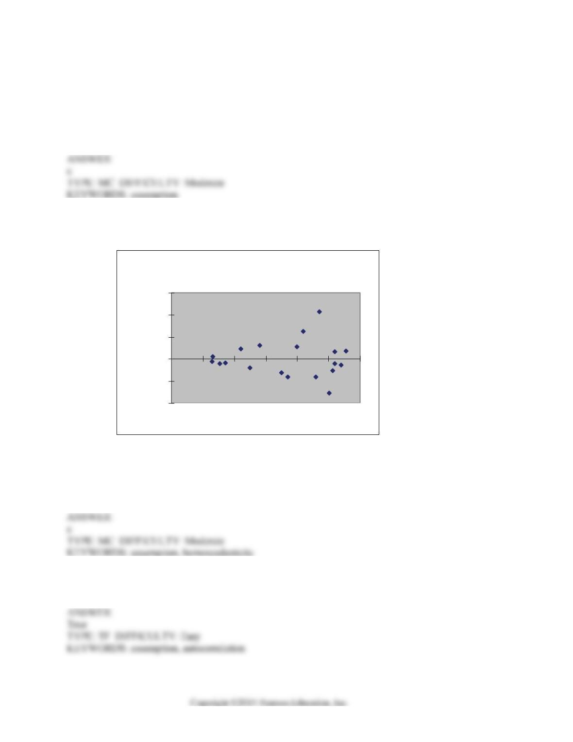
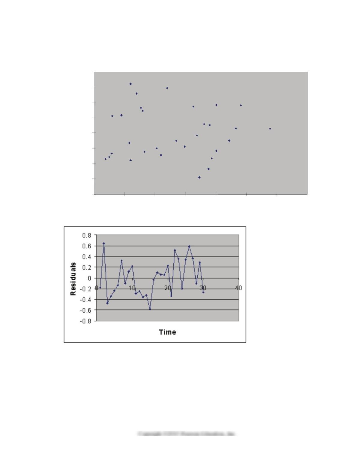
97. Based on the residual plot below, you will conclude that there might be a violation of which of
the following assumptions.
a) Linearity of the relationship
b) Normality of errors
c) Homoscedasticity
d) Independence of errors
98. True or False: Data that exhibit an autocorrelation effect violate the regression assumption of
independence.
Footage Residual Plot
-4000
-2000
0
2000
4000
6000
0 1,000 2,000 3,000 4,000 5,000 6,000
Footage
Residuals
Simple Linear Regression 13-25
99. True or False: The Durbin-Watson D statistic is used to check the assumption of normality.
100. If the residuals in a regression analysis of time-ordered data are not correlated, the value of the
Durbin-Watson D statistic should be near __________.
101. The residuals represent
a) the difference between the actual Y values and the mean of Y.
b) the difference between the actual Y values and the predicted Y values.
c) the square root of the slope.
d) the predicted value of Y for the average X value.
102. If the plot of the residuals is fan shaped, which assumption is violated?
a) Normality.
b) Homoscedasticity.
c) Independence of errors.
d) No assumptions are violated, the graph should resemble a fan.
103. What do we mean when we say that a simple linear regression model is “statistically” useful?
a) All the statistics computed from the sample make sense.
b) The model is an excellent predictor of Y.
c) The model is “practically” useful for predicting Y.
d) The model is a better predictor of Y than the sample mean, Y .
13-26 Simple Linear Regression
104. If the correlation coefficient (r) = 1.00, then
a) the Y-intercept (b0) must equal 0.
b) the explained variation equals the unexplained variation.
c) there is no unexplained variation.
d) there is no explained variation.
105. If the correlation coefficient (r) = 1.00, then
a) all the data points must fall exactly on a straight line with a slope that equals 1.00.
b) all the data points must fall exactly on a straight line with a negative slope.
c) all the data points must fall exactly on a straight line with a positive slope.
d) all the data points must fall exactly on a horizontal straight line with a zero slope.
106. Assuming a linear relationship between X and Y, if the coefficient of correlation (r) equals
– 0.30,
a) there is no correlation.
b) the slope (b1) is negative.
c) variable X is larger than variable Y.
d) the variance of X is negative.
107. Testing for the existence of correlation is equivalent to
a) testing for the existence of the slope (
β
1).
b) testing for the existence of the Y-intercept (
β
0).
c) the confidence interval estimate for predicting Y.
d) None of the above.
Simple Linear Regression 13-27
108. The strength of the linear relationship between two numerical variables may be measured by
the
a) scatter plot.
b) coefficient of correlation.
c) slope.
d) Y-intercept.
109. In a simple linear regression problem, r and b1
a) may have opposite signs.
b) must have the same sign.
c) must have opposite signs.
d) are equal.
110. The sample correlation coefficient between X and Y is 0.375. It has been found out that the p–
value is 0.256 when testing 0:0H
ρ
= against the two-sided alternative 1:0H
ρ
≠. To test
0:0H
ρ
= against the one-sided alternative 1:0H
ρ
< at a significance level of 0.1, the p-value
is
a) 0.256/2
b) (0.256)(2)
c) 1-0.256
d) 1-0.256/2
13-28 Simple Linear Regression
111. The sample correlation coefficient between X and Y is 0.375. It has been found out that the p–
value is 0.256 when testing 0:0H
ρ
= against the two-sided alternative 1:0H
ρ
≠. To test
0:0H
ρ
= against the one-sided alternative 1:0H
ρ
> at a significance level of 0.1, the p-value
is
a) 0.256 / 2
b)
()
0.256 2
c) 1 0.256−
d) 1 0.256 / 2−
112. The sample correlation coefficient between X and Y is 0.375. It has been found out that the p–
value is 0.256 when testing 0:0H
ρ
= against the one-sided alternative 1:0H
ρ
>. To test
0:0H
ρ
= against the two-sided alternative 1:0H
ρ
≠ at a significance level of 0.1, the p-value
is
a) 0.256 / 2
b)
()()
2256.0
c) 1 0.256−
d) 1 0.256 / 2−
113. The sample correlation coefficient between X and Y is 0.375. It has been found out that the p–
value is 0.744 when testing 0:0H
ρ
= against the one-sided alternative 1:0H
ρ
<. To test
0:0H
ρ
= against the two-sided alternative 1:0H
ρ
≠ at a significance level of 0.1, the p-value
is
a) 0.744 / 2
b)
()()
2744.0
c) 1 0.744−
d)
()()
2744.01−
Simple Linear Regression 13-29
114. If you wanted to find out if alcohol consumption (measured in fluid oz.) and grade point
average on a 4-point scale are linearly related, you would perform a
a. 2
χ
test for the difference in two proportions.
b. 2
χ
test for independence.
c. a Z test for the difference in two proportions.
d. a t test for a correlation coefficient.
115. True or False: When r = – 1, it indicates a perfect relationship between X and Y.
SCENARIO 13-7
An investment specialist claims that if one holds a portfolio that moves in the opposite direction to the
market index like the S&P 500, then it is possible to reduce the variability of the portfolio’s return. In
other words, one can create a portfolio with positive returns but less exposure to risk.
A sample of 26 years of S&P 500 index and a portfolio consisting of stocks of private prisons, which
are believed to be negatively related to the S&P 500 index, is collected. A regression analysis was
performed by regressing the returns of the prison stocks portfolio (Y) on the returns of S&P 500 index
(X) to prove that the prison stocks portfolio is negatively related to the S&P 500 index at a 5% level
of significance. The results are given in the following EXCEL output.
Coefficients Standard Error T Stat P-value
Intercept 4.8660 0.3574 13.6136 0.0000
S&P -0.5025 0.0716 -7.0186 0.0000
116. Referring to Scenario 13-7, to test whether the prison stocks portfolio is negatively related to
the S&P 500 index, the appropriate null and alternative hypotheses are, respectively,
a) 01
:0 vs. :0HH
ρρ
≥<
b) 01
: 0 vs. : 0HH
ρρ
≤>
c) 01
: 0 vs. : 0Hr Hr≥<
d) 01
: 0 vs. : 0Hr Hr≤>
13-30 Simple Linear Regression
117. Referring to Scenario 13-7, to test whether the prison stocks portfolio is negatively related to
the S&P 500 index, the measured value of the test statistic is
a) -7.019
b) -0.503
c) 0.072
d) 0.357
118. Referring to Scenario 13-7, to test whether the prison stocks portfolio is negatively related to
the S&P 500 index, the p-value of the associated test statistic is ______
119. Referring to Scenario 13-7, which of the following will be a correct conclusion?
a) You cannot reject the null hypothesis and, therefore, conclude that there is sufficient
evidence to show that the prisons stock portfolio and S&P 500 index are negatively
related.
b) You can reject the null hypothesis and, therefore, conclude that there is sufficient
evidence to show that the prisons stock portfolio and S&P 500 index are negatively
related.
c) You cannot reject the null hypothesis and, therefore, conclude that there is insufficient
evidence to show that the prisons stock portfolio and S&P 500 index are negatively
related.
d) You can reject the null hypothesis and conclude that there is insufficient evidence to
show that the prisons stock portfolio and S&P 500 index are negatively related.
Simple Linear Regression 13-31
SCENARIO 13-8
It is believed that GPA (grade point average, based on a four point scale) should have a positive linear
relationship with ACT scores. Given below is the Excel output for predicting GPA using ACT scores
based a data set of 8 randomly chosen students from a Big-Ten university.
Regressing GPA on ACT
Regression Statistics
Multiple R 0.7598
R Square 0.5774
Adjusted R Square 0.5069
Standard Error 0.2691
Observations 8
ANOVA
df SS MS F Significance F
Regression 1 0.5940 0.5940 8.1986 0.0286
Residual 6 0.4347 0.0724
Total 7 1.0287
Coefficients Standard Error t Stat P-value Lower 95% Upper 95%
Intercept 0.5681 0.9284 0.6119 0.5630 -1.7036 2.8398
ACT 0.1021 0.0356 2.8633 0.0286 0.0148 0.1895
120. Referring to Scenario 13-8, the interpretation of the coefficient of determination in this
regression is
a) 57.74% of the total variation of ACT scores can be explained by GPA.
b) ACT scores account for 57.74% of the total fluctuation in GPA.
c) GPA accounts for 57.74% of the variability of ACT scores.
d) None of the above.
121. Referring to Scenario 13-8, the value of the measured test statistic to test whether there is any
linear relationship between GPA and ACT is
a) 0.0356
b) 0.1021
c) 0.7598
d) 2.8633
13-32 Simple Linear Regression
122. Referring to Scenario 13-8, what is the predicted value of GPA when ACT = 20?
a. 2.61
b. 2.66
c. 2.80
d. 3.12
123. Referring to Scenario 13-8, what are the decision and conclusion on testing whether there is any
linear relationship at 1% level of significance between GPA and ACT scores?
a) Do not reject the null hypothesis; hence there is insufficient evidence to show that ACT
scores and GPA are linearly related.
b) Reject the null hypothesis; hence there is insufficient evidence to show that ACT scores
and GPA are linearly related.
c) Do not reject the null hypothesis; hence there is sufficient evidence to show that ACT
scores and GPA are linearly related.
d) Reject the null hypothesis; hence there is sufficient evidence to show that ACT scores
and GPA are linearly related.
124. Referring to Scenario 13-8, the value of the measured (observed) test statistic of the F-test for
01
: 0 vs. : 0HH
ββ
11
=≠
a) may be negative.
b) is always positive.
c) is always negative.
d) has the same sign as the corresponding t test statistic.

Simple Linear Regression 13-33
SCENARIO 13-9
It is believed that, the average numbers of hours spent studying per day (HOURS) during
undergraduate education should have a positive linear relationship with the starting salary (SALARY,
measured in thousands of dollars per month) after graduation. Given below is the Excel output for
predicting starting salary (Y) using number of hours spent studying per day (X) for a sample of 51
students. NOTE: Only partial output is shown.
Regression Statistics
Multiple R 0.8857
R Square 0.7845
Adjusted R Square 0.7801
Standard Error 1.3704
Observations 51
ANOVA
df SS MS F Significance F
Regression 1 335.0472 335.0473 178.3859
Residual 1.8782
Total 50 427.0798
Coefficients
Standard
Error t Stat P-value Lower 95% Upper 95%
Intercept -1.8940 0.4018 -4.7134 0.0000 -2.7015 -1.0865
Hours 0.9795 0.0733 13.3561 0.0000 0.8321 1.1269
Note: 05
2.051 05 2.051*10E−
−= and 18
5.944 18 5.944 *10E−
−= .
125. Referring to Scenario 13-9, the estimated change in mean salary (in thousands of dollars) as a
result of spending an extra hour per day studying is
a. -1.8940
b. 0.7845
c. 0.9795
d. 335.0473
13-34 Simple Linear Regression
126. Referring to Scenario 13-9, the value of the measured t-test statistic to test whether mean
SALARY depends linearly on HOURS is
a) -4.7134
b) -1.8940
c) 0.9795
d) 13.3561
127. Referring to Scenario 13-9, the p-value of the measured F-test statistic to test whether HOURS
affects SALARY is _____.
128. Referring to Scenario 13-9, the degrees of freedom for the F test on whether HOURS affects
SALARY are
a) 1, 49
b) 1, 50
c) 49, 1
d) 50, 1
129. Referring to Scenario 13-9, the error sum of squares (SSE) of the above regression is
a) 1.878215
b) 92.0325465
c) 335.047257
d) 427.079804
Simple Linear Regression 13-35
130. Referring to Scenario 13-9, the 90% confidence interval for the average change in SALARY (in
thousands of dollars) as a result of spending an extra hour per day studying is
a) wider than [-2.70159, -1.08654].
b) narrower than [-2.70159, -1.08654].
c) wider than [0.8321927, 1.12697].
d) narrower than [0.8321927, 1.12697].
131. Referring to Scenario 13-9, to test the claim that SALARY depends positively on HOURS
against the null hypothesis that SALARY does not depend linearly on HOURS, the p-value of the
test statistic is _____.
132. True or False: A zero population correlation coefficient between a pair of random variables
means that there is no linear relationship between the random variables.
133. True or False: You give a pre-employment examination to your applicants. The test is scored
from 1 to 100. You have data on their sales at the end of one year measured in dollars. You want
to know if there is any linear relationship between pre-employment examination score and sales.
An appropriate test to use is the t test of the population correlation coefficient.
13-36 Simple Linear Regression
134. The width of the prediction interval for the predicted value of Y is dependent on
a) the standard error of the estimate.
b) the value of X for which the prediction is being made.
c) the sample size.
d) All of the above.
135. True or False: The confidence interval for the mean of Y is always narrower than the prediction
interval for an individual response Y given the same data set, X value, and confidence level.
SCENARIO 13-10
The management of a chain electronic store would like to develop a model for predicting the weekly
sales (in thousand of dollars) for individual stores based on the number of customers who made
purchases. A random sample of 12 stores yields the following results:
Customers Sales (Thousands of Dollars)
907 11.20
926 11.05
713 8.21
741 9.21
780 9.42
898 10.08
510 6.73
529 7.02
460 6.12
872 9.52
650 7.53
603 7.25
Simple Linear Regression 13-37
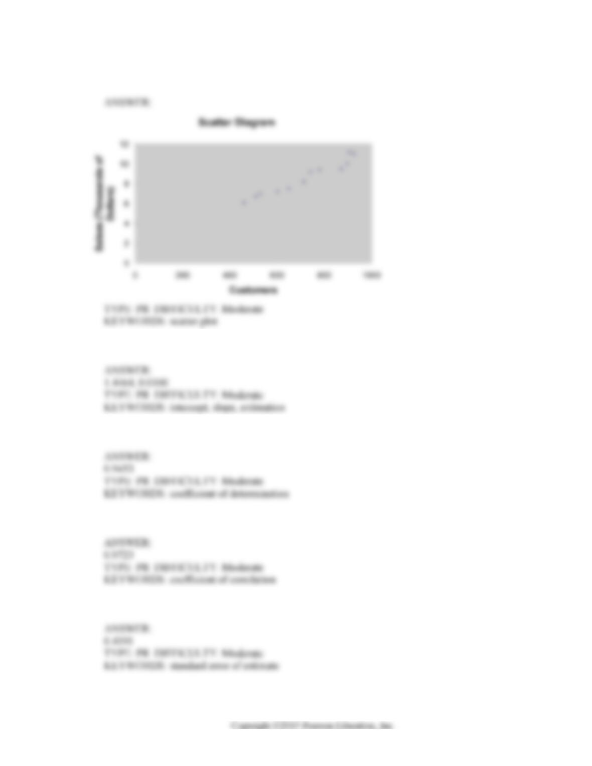
136. Referring to Scenario 13-10, generate the scatter plot.
137. Referring to Scenario 13-10, what are the values of the estimated intercept and slope?
138. Referring to Scenario 13-10, what is the value of the coefficient of determination?
139. Referring to Scenario 13-10, what is the value of the coefficient of correlation?
140. Referring to Scenario 13-10, what is the value of the standard error of the estimate?
13-38 Simple Linear Regression
141. Referring to Scenario 13-10, which is the correct null hypothesis for testing whether the
number of customers who make a purchase affects weekly sales?
a) 00
:0H
β
=
b) 01
:0H
β
=
c) 0:0H
μ
=
d) 0:0H
π
=
142. Referring to Scenario 13-10, what is the value of the t test statistic when testing whether the
number of customers who make a purchase affects weekly sales?
143. Referring to Scenario 13-10, what are the degrees of freedom of the t test statistic when testing
whether the number of customers who make a purchase affects weekly sales?
144. Referring to Scenario 13-10, what is the p-value of the t test statistic when testing whether the
number of customers who make a purchase affects weekly sales?
145. True or False: Referring to Scenario 13-10, the null hypothesis for testing whether the number
of customers who make a purchase effects weekly sales cannot be rejected if a 1% probability of
committing a type I error is desired.
Simple Linear Regression 13-39
146. True or False: Referring to Scenario 13-10, the mean weekly sales will increase by an estimated
$0.01 for each additional purchasing customer.
147. True or False: Referring to Scenario 13-10, the mean weekly sales will increase by an estimated
$10 for each additional purchasing customer.
148. True or False: Referring to Scenario 13-10, 93.98% of the total variation in weekly sales can be
explained by the variation in the number of customers who make purchases.
149. Referring to Scenario 13-10, what are the degrees of freedom of the F test statistic when testing
whether the number of customers who make purchases is a good predictor for weekly sales?
150. Referring to Scenario 13-10, what is the value of the F test statistic when testing whether the
number of customers who make purchases is a good predictor for weekly sales?
151. Referring to Scenario 13-10, what is the p-value of the F test statistic when testing whether the
number of customers who make purchases is a good predictor for weekly sales?
13-40 Simple Linear Regression
152. True or False: Referring to Scenario 13-10, the p-value of the t test and F test should be the
same when testing whether the number of customers who make purchases is a good predictor for
weekly sales.
153. True or False: Referring to Scenario 13-10, the value of the t test statistic and F test statistic
should be the same when testing whether the number of customers who make purchases is a good
predictor for weekly sales.
154. True or False: Referring to Scenario 13-10, the value of the F test statistic equals the square of
the t test statistic when testing whether the number of customers who make purchases is a good
predictor for weekly sales.
155. Referring to Scenario 13-10, generate the residual plot.
Simple Linear Regression 13-41
156. Referring to Scenario 13-10, the residual plot indicates possible violation of which
assumptions?
a) Linearity of the relationship
b) Homoscedasticity
c) Autocorrelation
d) Normality
157. True or False: Referring to Scenario 13-10, it is inappropriate to compute the Durbin-Watson
statistic and test for autocorrelation in this case.
158. Referring to Scenario 13-10, construct a 95% confidence interval for the change in mean
weekly sales when the number of customers who make purchases increases by one.
159. Referring to Scenario 13-10, construct a 95% confidence interval for the mean weekly sales
when the number of customers who make purchases is 600.
160. Referring to Scenario 13-10, construct a 95% prediction interval for the weekly sales of a store
that has 600 purchasing customers.
13-42 Simple Linear Regression
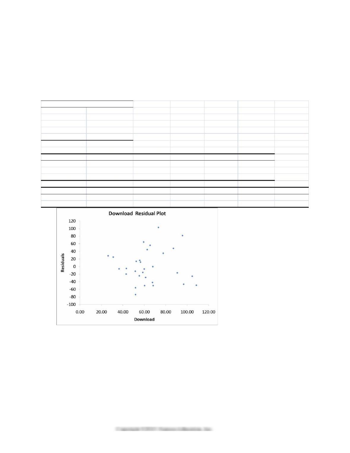
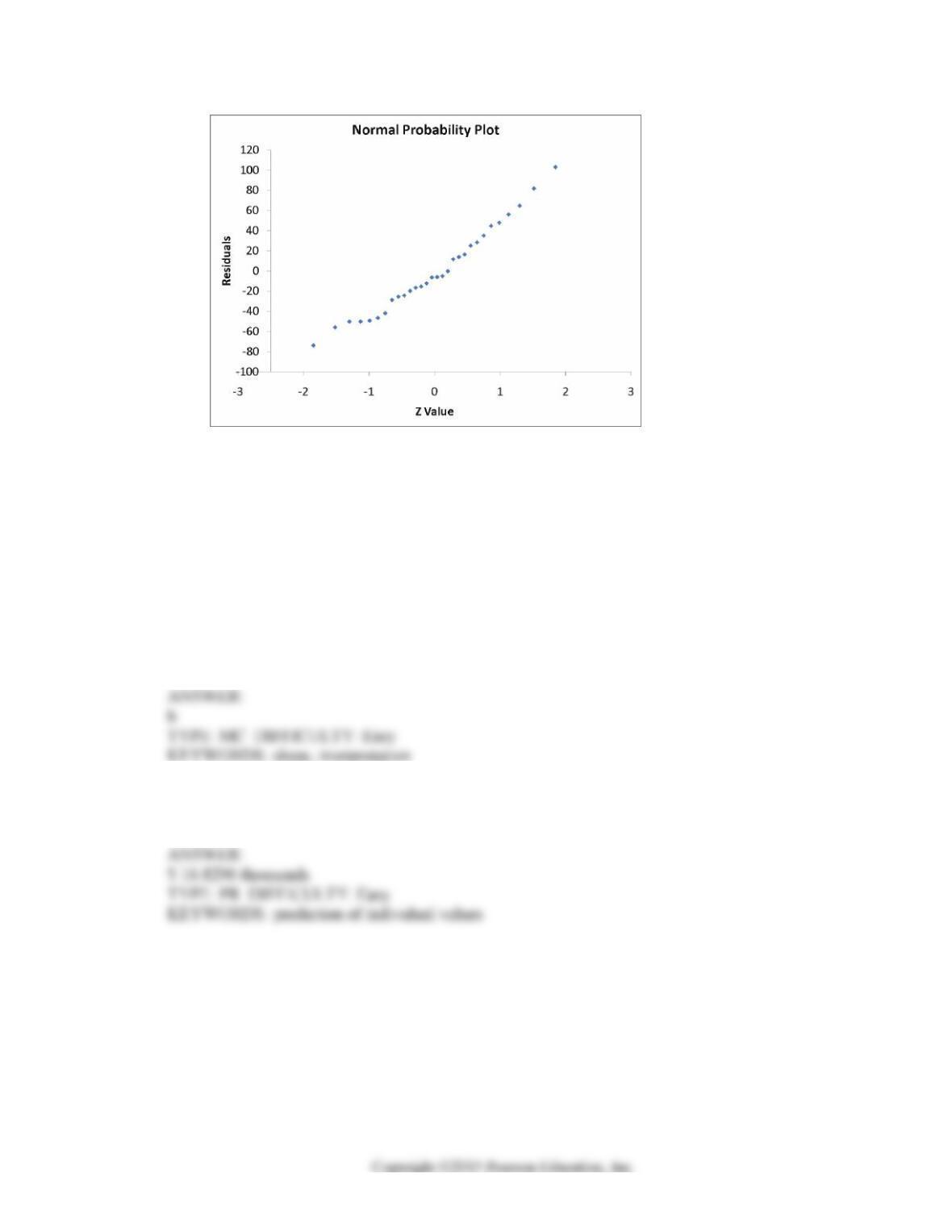
SCENARIO 13-11
A computer software developer would like to use the number of downloads (in thousands) for the trial
version of his new shareware to predict the amount of revenue (in thousands of dollars) he can make
on the full version of the new shareware. Following is the output from a simple linear regression
along with the residual plot and normal probability plot obtained from a data set of 30 different
sharewares that he has developed:
Regression Statistics
Multiple R 0.8691
R Square 0.7554
Adjusted R Square 0.7467
Standard Error 44.4765
Observations 30.0000
ANOVA
df SS MS F Significance F
Regression 1 171062.9193 171062.9193 86.4759 0.0000
Residual 28 55388.4309 1978.1582
Total 29 226451.3503
Coefficients Standard Error t Stat P-value Lower 95% Upper 95%
Intercept -95.0614 26.9183 -3.5315 0.0015 -150.2009 -39.9218
Download 3.7297 0.4011 9.2992 0.0000 2.9082 4.5513
Simple Linear Regression 13-43
161. Referring to Scenario 13-11, which of the following is the correct interpretation for the slope
coefficient?
a) For each decrease of 1 thousand downloads, the expected revenue is estimated to increase
by $ 3.7297 thousands.
b) For each increase of 1 thousand downloads, the expected revenue is estimated to increase
by $ 3.7297 thousands.
c) For each decrease of 1 thousand dollars in expected revenue, the expected number of
downloads is estimated to increase by 3.7297 thousands.
d) For each increase of 1 thousand dollars in expected revenue, the expected number of
downloads is estimated to increase by 3.7297 thousands.
162. Referring to Scenario 13-11, predict the revenue when the number of downloads is 30
thousands.
13-44 Simple Linear Regression
163. Referring to Scenario 13-11, which of the following is the correct interpretation for the
coefficient of determination?
a) 74.67% of the variation in revenue can be explained by the variation in the number of
downloads.
b) 75.54% of the variation in revenue can be explained by the variation in the number of
downloads.
c) 74.67% of the variation in the number of downloads can be explained by the variation in
revenue.
d) 75.54% of the variation in the number of downloads can be explained by the variation in
revenue.
164. Referring to Scenario 13-11, what is the standard error of estimate?
165. Referring to Scenario 13-11, what is the standard deviation around the regression line?
166. Referring to Scenario 13-11, which of the following assumptions appears to have been
violated?
a) Normality of error
b) Homoscedasticity
c) Independence of errors
d) None of the above
Simple Linear Regression 13-45
167. True or False: Referring to Scenario 13-11, the normality of error assumption appears to have
been violated.
168. True or False: Referring to Scenario 13-11, the homoscedasticity of error assumption appears to
have been violated.
169. True or False: Referring to Scenario 13-11, there appears to be autocorrelation in the residuals.
170. True or False: Referring to Scenario 13-11, the Durbin-Watson statistic is inappropriate for this
data set.
171. True or False: Referring to Scenario 13-11, the null hypothesis for testing whether there is a
linear relationship between revenue and the number of downloads is “There is no linear
relationship between revenue and the number of downloads”.
13-46 Simple Linear Regression
172. Referring to Scenario 13-11, which of the following is the correct null hypothesis for testing
whether there is a linear relationship between revenue and the number of downloads?
a) 01
:0Hb=
b) 01
:0Hb≠
c) 01
:0H
β
=
d) 01
:0H
β
≠
173. Referring to Scenario 13-11, which of the following is the correct alternative hypothesis for
testing whether there is a linear relationship between revenue and the number of downloads?
a) 11
:0Hb=
b) 11
:0Hb≠
c) 11
:0H
β
=
d) 11
:0H
β
≠
174. Referring to Scenario 13-11, what is the value of the test statistic for testing whether there is a
linear relationship between revenue and the number of downloads?
175. Referring to Scenario 13-11, what is the critical value for testing whether there is a linear
relationship between revenue and the number of downloads at a 5% level of significance?
176. Referring to Scenario 13-11, what is the p-value for testing whether there is a linear relationship
between revenue and the number of downloads at a 5% level of significance?
Simple Linear Regression 13-47
177. True or False: Referring to Scenario 13-11, the null hypothesis that there is no linear
relationship between revenue and the number of downloads should be rejected at a 5% level of
significance.
178. True or False: Referring to Scenario 13-11, there is sufficient evidence that revenue and the
number of downloads are linearly related at a 5% level of significance.
179. Referring to Scenario 13-11, what arethe lower and upper limits of the 95% confidence interval
estimate for population slope?
180. Referring to Scenario 13-11, what arethe lower and upper limits of the 95% confidence interval
estimate for the mean change in revenue as a result of a one thousand increase in the number of
downloads?

13-48 Simple Linear Regression
SCENARIO 13-12
The manager of the purchasing department of a large saving and loan organization would like to
develop a model to predict the amount of time (measured in hours) it takes to record a loan
application. Data are collected from a sample of 30 days, and the number of applications recorded and
completion time in hours is recorded. Below is the regression output:
Regression Statistics
Multiple R 0.9447
R Square 0.8924
Adjusted R
Square
0.8886
Standard
Error
0.3342
Observations 30
ANOVA
df SS MS F Significance
F
Regression 1 25.9438 25.9438 232.2200 4.3946E-15
Residual 28 3.1282 0.1117
Total 29 29.072
Coefficients Standard
Error
t Stat P-value Lower 95% Upper 95%
Intercept 0.4024 0.1236 3.2559 0.0030 0.1492 0.6555
Applications
Recorded
0.0126 0.0008 15.2388 0.0000 0.0109 0.0143
Simple Linear Regression 13-49
Applications Recorded Residual Plot
–
–
–
–
0
0.
0.
0.
0.
0 5 10 150 20 25 30 350
Loan Applications Recorded
Residuals
13-50 Simple Linear Regression
181. Referring to Scenario 13-12, the estimated mean amount of time it takes to record one
additional loan application is
a) 0.4024 fewer hours
b) 0.4024 more hours
c) 0.0126 fewer hours
d) 0.0126 more hours
182. Referring to Scenario 13-12, the value of the measured t-test statistic to test whether the amount
of time depends linearly on the number of loan applications recorded is
a) 0.8924
b) 3.2559
c) 15.2388
d) 232.2200
183. Referring to Scenario 13-12, the p-value of the measured F-test statistic to test whether the
number of loan applications recorded affects the amount of time is _____.
184. Referring to Scenario 13-12, the p-value of the measured t-test statistic to test whether the
number of loan applications recorded affects the amount of time is _____.
Simple Linear Regression 13-51
185. Referring to Scenario 13-12, the degrees of freedom for the F test on whether the number of
load applications recorded affects the amount of time are
a) 1, 28
b) 1, 29
c) 28, 1
d) 29, 1
186. Referring to Scenario 13-12, the degrees of freedom for the t test on whether the number of
loan applications recorded affects the amount of time are
a) 1
b) 28
c) 29
d) 30
187. Referring to Scenario 13-12, the error sum of squares (SSE) of the above regression is
a) 0.1117
b) 3.1282
c) 25.9438
d) 29.0720
188. Referring to Scenario 13-12, the 90% confidence interval for the mean change in the amount of
time needed as a result of recording one additional loan application is
a) wider than [0.1492, 0.6555].
b) narrower than [0.1492, 0.6555].
c) wider than [0.0109, 0.0143].
d) narrower than [0.0109, 0.0143].
13-52 Simple Linear Regression
189. True or False: Referring to Scenario 13-12, you can be 95% confident that the mean amount of
time needed to record one additional loan application is somewhere between 0.0109 and 0.0143
hours.
190. True or False: Referring to Scenario 13-12, there is a 95% probability that the mean amount of
time needed to record one additional loan application is somewhere between 0.0109 and 0.0143
hours.
191. True or False: Referring to Scenario 13-12, there is sufficient evidence that the amount of time
needed linearly depends on the number of loan applications at a 5% level of significance.
192. True or False: Referring to Scenario 13-12, there is sufficient evidence that the amount of time
needed linearly depends on the number of loan applications at a 1% level of significance.
193. Referring to Scenario 13-12, to test the claim that the mean amount of time depends positively
on the number of loan applications recorded against the null hypothesis that the mean amount of
time does not depend linearly on the number of invoices processed, the p-value of the test statistic
is ____.
Simple Linear Regression 13-53
194. Referring to Scenario 13-12, predict the amount of time it would take to process 150 invoices.
195. Referring to Scenario 13-12, what percentage of the variation in the amount of time needed can
be explained by the variation in the number of invoices processed?
196. True or False: Referring to Scenario 13-12, the model appears to be adequate based on the
residual analyses.
197. Referring to Scenario 13-12, what are the critical values of the Durbin-Watson test statistic
using the 5% level of significance to test for evidence of positive autocorrelation?
198. True or False: Referring to Scenario 13-12, there is no evidence of positive autocorrelation if
the Durbin-Watson test statistic is found to be 1.78.

13-54 Simple Linear Regression
SCENARIO 13-13
In this era of tough economic conditions, voters increasingly ask the question: “Is the educational
achievement level of students dependent on the amount of money the state in which they reside
spends on education?” The partial computer output below is the result of using spending per student
($) as the independent variable and composite score which is the sum of the math, science and
reading scores as the dependent variable on 35 states that participated in a study. The table includes
only partial results.
Regression Statistics
Multiple R 0.3122
R Square 0.0975
Adjusted R
Square
0.0701
Standard
Error
26.9122
Observations 35
ANOVA
df SS MS F
Regression 1 2581.5759
Residual 724.2674
Total 34 26482.4000
Coefficients Standard Error t Stat P-value
Intercept 595.540251 22.115176
Spending per
Student ($) 0.007996 0.004235
199. Referring to Scenario 13-13, if the state decides to spend 1,000 dollar more per student, the
estimated change in mean composite score is _________.
200. Referring to Scenario 13-13, the value of the measured t-test statistic to test whether composite
score depends linearly on spending per student is ________.
Simple Linear Regression 13-55
201. Referring to Scenario 13-13, the p-value of the measured t-test statistic to test whether
composite score depends linearly on spending per student is ________.
202. Referring to Scenario 13-13, the decision on the test of whether composite score depends
linearly on spending per student using a 10% level of significance is to ________ (reject or not
reject) 0
H
.
203. Referring to Scenario 13-13, the conclusion on the test of whether composite score depends
linearly on spending per student using a 10% level of significance is _________
a) There is not enough evidence that composite score does not depend linearly on spending
per student.
b) There is enough evidence that composite score does not depend linearly on spending per
student.
c) There is not enough evidence that composite score depends linearly on spending per
student.
d) There is enough evidence that composite score depends linearly on spending per student.
204. Referring to Scenario 13-13, the p-value of the measured F-test statistic to test whether
spending per student affects composite score is ________.
205. Referring to Scenario 13-13, the degrees of freedom for the F test on whether spending per
student affects composite score are _________.
13-56 Simple Linear Regression
206. Referring to Scenario 13-13, the value of the F test on whether spending per student affects
composite score is _________.
207. Referring to Scenario 13-13, the critical value at 5% level of significance of the F test on
whether spending per student affects composite score is _________.
208. Referring to Scenario 13-13, the decision on the test of whether spending per student affects
composite score using a 5% level of significance is to ________ (reject or not reject) 0
H
.
209. Referring to Scenario 13-13, the conclusion on the test of whether spending per student affects
composite score using a 5% level of significance is
a) There is not enough evidence that spending per student affects composite score.
b) There is enough evidence that spending per student affects composite score.
c) There is not enough evidence that spending per student does not affect composite score.
d) There is enough evidence that spending per student does not affect composite score.
210. Referring to Scenario 13-13, the error sum of squares (SSE) of the above regression is _____.
211. Referring to Scenario 13-13, the regression mean square (MSR) of the above regression is
_____.
Simple Linear Regression 13-57
212. Referring to Scenario 13-13, what percentage of the variation in composite score can be
explained by the variation in spending per student?
213. Referring to Scenario 13-13, what is the standard deviation of the composite score around the
regression line?