12. Shown below is a 2 3 contingency table with observed values from a sample of 500. At 95%
confidence, test for independence of the row and column factors.
Column Factor
Row Factor
x
y
Z
A
40
50
110
B
60
100
140
13. A sample of 150 individuals (males and females) was surveyed, and the individuals were asked to
indicate their yearly incomes. The results of the survey are shown below.
Income Category
Male
Female
Category 1: $20,000 up to $40,000
10
30
Category 2: $40,000 up to $60,000
35
15
Category 3: $60,000 up to $80,000
15
45
Test at = 0.05 to determine if the yearly income is independent of the gender.
14. A group of 2000 individuals from 3 different cities were asked whether they owned a foreign or a
domestic car. The following contingency table shows the results of the survey.
City
Type of Car
Detroit
Atlanta
Denver
Total
Domestic
80
200
520
800
Foreign
120
600
480
1,200
Total
200
800
1,000
2,000
At = 0.05, test to determine if the type of car purchased is independent of the city in which the
purchasers live.
15. Dr. Ross’ diet pills are supposed to cause significant weight loss. The following table shows the results
of a recent study where some individuals took the diet pills and some did not.
Diet Pills
No Diet Pills
Total
No Weight Loss
80
20
100
Weight Loss
100
100
200
Total
180
120
300
With 95% confidence, test to see if losing weight is dependent on taking the diet pills.
16. Five hundred randomly selected automobile owners were questioned on the main reason they had
purchased their current automobile. The results are given below.
Main Reason Purchased
Styling
Engineering
Fuel Economy
Total
Male
70
130
150
350
Female
30
20
100
150
Total
100
150
250
500
a.
State the null and alternative hypotheses for a contingency table test.
b.
State the decision rule, using a .10 level of significance.
c.
Calculate the chi-square test statistic.
d.
Give your conclusion for this test.
a.
Do not reject H0 if chi-square 4.60517
Reject H0 if chi-square > 4.60517
c.
31.746
17. A group of 500 individuals were asked to cast their votes regarding a particular issue of the Equal
Rights Amendment. The following contingency table shows the results of the votes:
Vote Cast
Gender
Favor
Undecided
Oppose
Total
Female
180
80
40
300
Male
150
20
30
200
Total
330
100
70
500
Test at = .05 to determine if the votes cast were independent of the gender of the individuals.
18. One thousand managers with degrees in business administration indicated their fields of concentration
as shown below.
Major
Top Management
Middle Management
Total
Management
300
200
500
Marketing
200
0
200
Accounting
100
200
300
Total
600
400
1,000
Test at = .01 to determine if the position in management is independent of the major of
concentration.
19. From a poll of 800 television viewers, the following data have been accumulated as to their levels of
education and their preference of television stations:
Level of Educational
High School
Bachelor
Graduate
Total
Public Broadcasting
150
150
100
400
Commercial Stations
50
250
100
400
Total
200
400
200
800
Test at = .05 to determine if the selection of a TV station is dependent upon the level of education.
20. The data below represents the fields of specialization for a randomly selected sample of undergraduate
students. Test to determine whether there is a significant difference in the fields of specialization
between regions of the country. Use a .05 level of significance.
Region of United States
Specialization
Northeast
Midwest
South
West
Total
Business
54
65
28
93
240
Engineering
15
24
8
33
80
Liberal Arts
65
84
33
98
280
Fine Arts
13
15
7
25
60
Health Sciences
3
12
4
21
40
Total
150
200
80
270
700
a.
State the critical value of the chi-square random variable for this test of independence of
categories.
b.
Calculate the value of the test statistic.
c.
What is the conclusion for this test?
21.0261
b.
8.674
c.
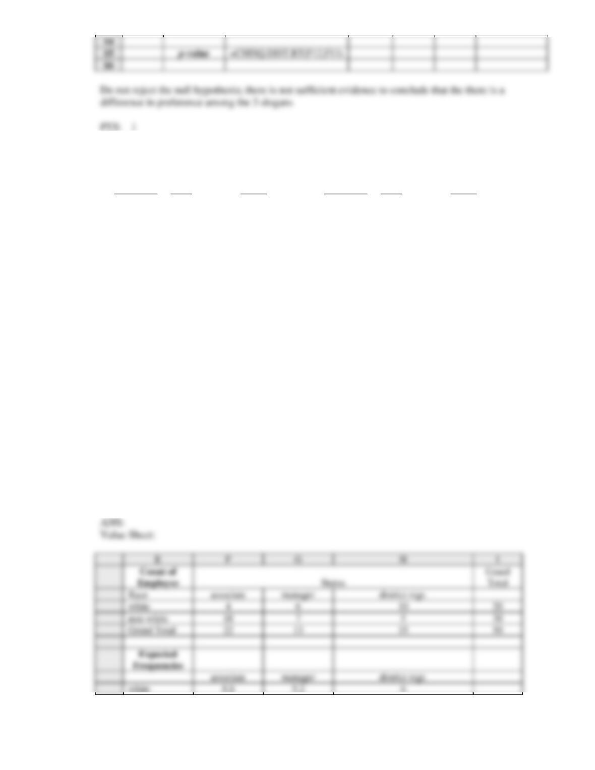
Do not reject the null hypothesis that fields of specialization and region are independent.
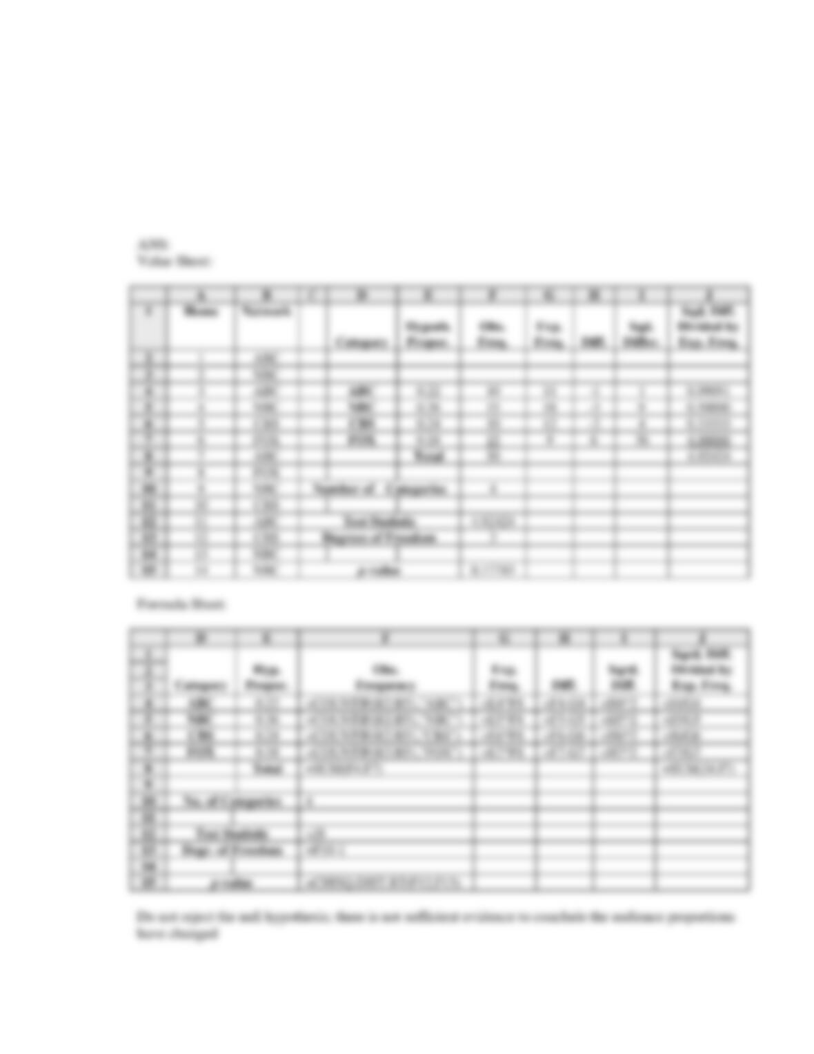
21. During “sweeps week” last year, the viewing audience was distributed as follows: 36% NBC, 22%
ABC, and 24% CBS, and 18% FOX. This year during “sweeps week” a sample of 50 homes yielded
the following data. Use Excel to test at = .05 to determine if the audience proportions have changed.
ABC
FOX
ABC
FOX
ABC
ABC
CBS
NBC
FOX
FOX
NBC
ABC
CBS
ABC
NBC
NBC
NBC
CBS
FOX
ABC
ABC
FOX
NBC
CBS
CBS
NBC
NBC
ABC
FOX
FOX
NBC
NBC
NBC
NBC
FOX
ABC
FOX
NBC
FOX
CBS
CBS
CBS
FOX
FOX
NBC
CBS
FOX
CBS
FOX
NBC
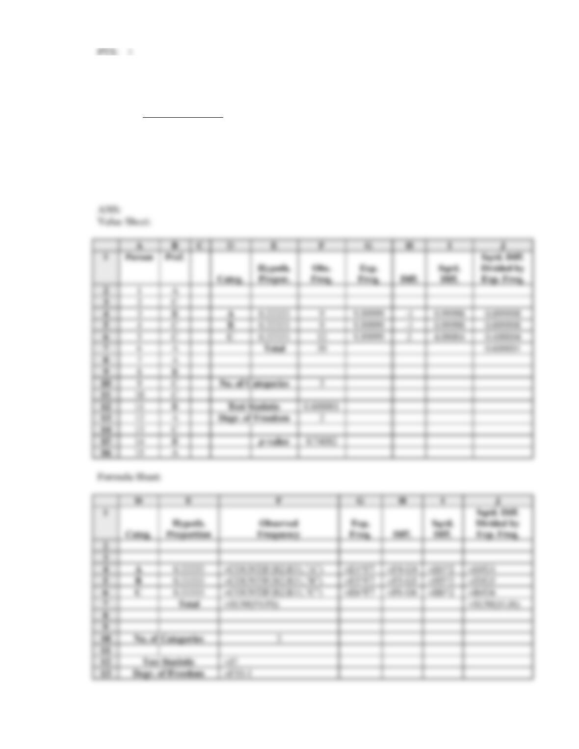
22. Members of a focus group stated their preferences between three possible slogans. The results follow.
Use Excel to test at = .05 to determine any difference in preference among the three slogans.
Slogan Preferences
A
A
C
C
B
C
B
B
A
A
B
C
A
B
C
C
C
C
B
B
C
B
C
C
A
A
A
C
A
B
23. A study of wage discrimination at a local store compared employees’ race and their status. Partial
results of the study follow. Use Excel and test at = .05 to determine if race is independent of status.
Employee
Race
Status
Employee
Race
Status
1
white
manager
26
non-white
associate
2
non-white
associate
27
white
district mgr.
3
white
district mgr.
28
non-white
manager
4
white
manager
29
white
associate
5
white
manager
30
non-white
district mgr.
6
non-white
associate
31
non-white
district mgr.
7
non-white
associate
32
white
district mgr.
8
white
associate
33
white
district mgr.
9
non-white
associate
34
non-white
associate
10
white
manager
35
white
district mgr.
11
non-white
manager
36
non-white
associate
12
non-white
associate
37
non-white
manager
13
white
associate
38
non-white
associate
14
non-white
associate
39
white
district mgr.
15
white
district mgr.
40
non-white
associate
16
white
district mgr.
41
non-white
manager
17
non-white
associate
42
non-white
district mgr.
18
non-white
associate
43
white
manager
19
white
associate
44
white
district mgr.
20
non-white
manager
45
non-white
associate
21
white
district mgr.
46
non-white
associate
22
non-white
district mgr.
47
non-white
district mgr.
23
non-white
manager
48
white
manager
24
non-white
associate
49
non-white
manager
25
non-white
associate
50
non-white
associate
24. City planners are evaluating three proposed alternatives for relieving the growing traffic congestion on
a north-south highway in a booming city. The proposed alternatives are: (1) designate
high-occupancy vehicle (HOV) lanes on the existing highway, (2) construct a new, parallel highway,
and (3) construct a light (passenger) rail system.
In an analysis of the three proposals, a citizen group has raised the question of whether preferences for
the three alternatives differ among residents near the highway and non-residents. A test of
independence will address this question, with the hypotheses being:
H0: Proposal preference is independent of the residency status of the individual
Ha: Proposal preference is not independent of the residency status of the individual
A simple random sample of 500 individuals has been selected. A crosstabulation of the residency
statuses and proposal preferences of the individuals sampled is shown below.
PROPOSAL
Residency Status
HOV Lanes
New Highway
Light Rail
Nearby Resident
110
45
70
Distant Resident
140
75
60
Conduct a test of independence using
= .05 to address the question of whether residency status is
independent of the proposal preference.
25. Employee panel preferences for three proposed company logo designs follow.
Design A
Design B
Design C
78
59
66
Use
= .05 and test to determine any difference in preference among the three logo designs.
26. Shoppers were asked where they do their regular grocery shopping. The table below shows the
responses of the sampled shoppers. We are interested in determining if the proportions of females in
the three categories are different from each other.
Gender
Grocery
Chain
Discount
Store
Membership
Warehouse
Total
Female
230
80
100
410
Male
80
50
60
190
Total
310
130
160
600
a.
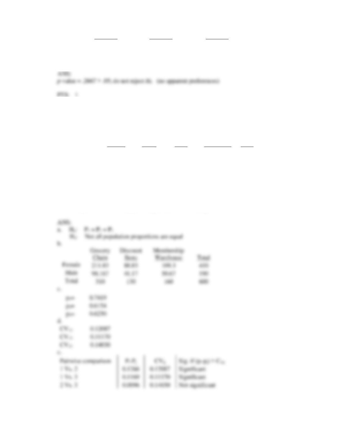
Provide the null and the alternative hypotheses.
b.
Determine the expected frequencies.
c.
Compute the sample proportions.
d.
Compute the critical values (CVij).
e.
Give your conclusions by providing numerical reasoning.
0.7419
0.6154
0.6250
Pairwise comparison
Sig. if (pi-pj) > Cvij
1 Vs. 2
Significant
1 Vs. 3
Significant
2 Vs. 3
Not significant
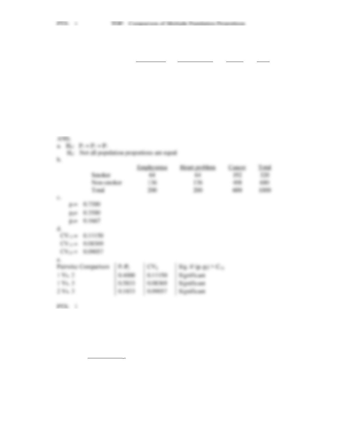
27. The following table shows the results of a study on smoking and three illnesses. We are interested in
determining if the proportions smokers in the three categories are different from each other.
Emphysema
Heart problem
Cancer
Total
Smoker
150
70
100
320
Non-smoker
50
130
500
680
Total
200
200
600
1000
a.
Provide the null and the alternative hypotheses.
b.
Determine the expected frequencies.
c.
Compute the sample proportions.
d.
Compute the critical values (CVij).
e.
Give your conclusions by providing numerical reasoning.
28. Prior to the start of the season, it was expected that audience proportions for the four major news
networks would be CBS 18.6%, NBC 12.5%, ABC 28.9% and BBC 40%. A recent sample of homes
yielded the following viewing audience data.
Observed
Frequencies (fi)
CBS
400
NBC
230
ABC
560
BBC
810
Total
2000
We want to determine whether or not the recent sample supports the expectations of the number of
homes of the viewing audience of the four networks.
a.
State the null and alternative hypotheses to be tested.
b.
Compute the test statistic.
c.
The null hypothesis is to be tested at 95% confidence. Determine the critical value for this
test.
d.
What do you conclude?
29. Prior to the start of the season, it was expected that audience proportions for the four major news
networks would be CBS 28%, NBC 35%, ABC 22% and BBC 15%. A recent sample of homes
yielded the following viewing audience data.
Network
Number of Homes
CBS
850
NBC
980
ABC
670
BBC
500
We want to determine whether or not the recent sample supports the expectations of the number of
homes of the viewing audience of the four networks.
a.
State the null and alternative hypotheses to be tested.
b.
Compute the test statistic.
c.
The null hypothesis is to be tested at 95% confidence. Determine the critical value for this
test.
d.
What do you conclude?
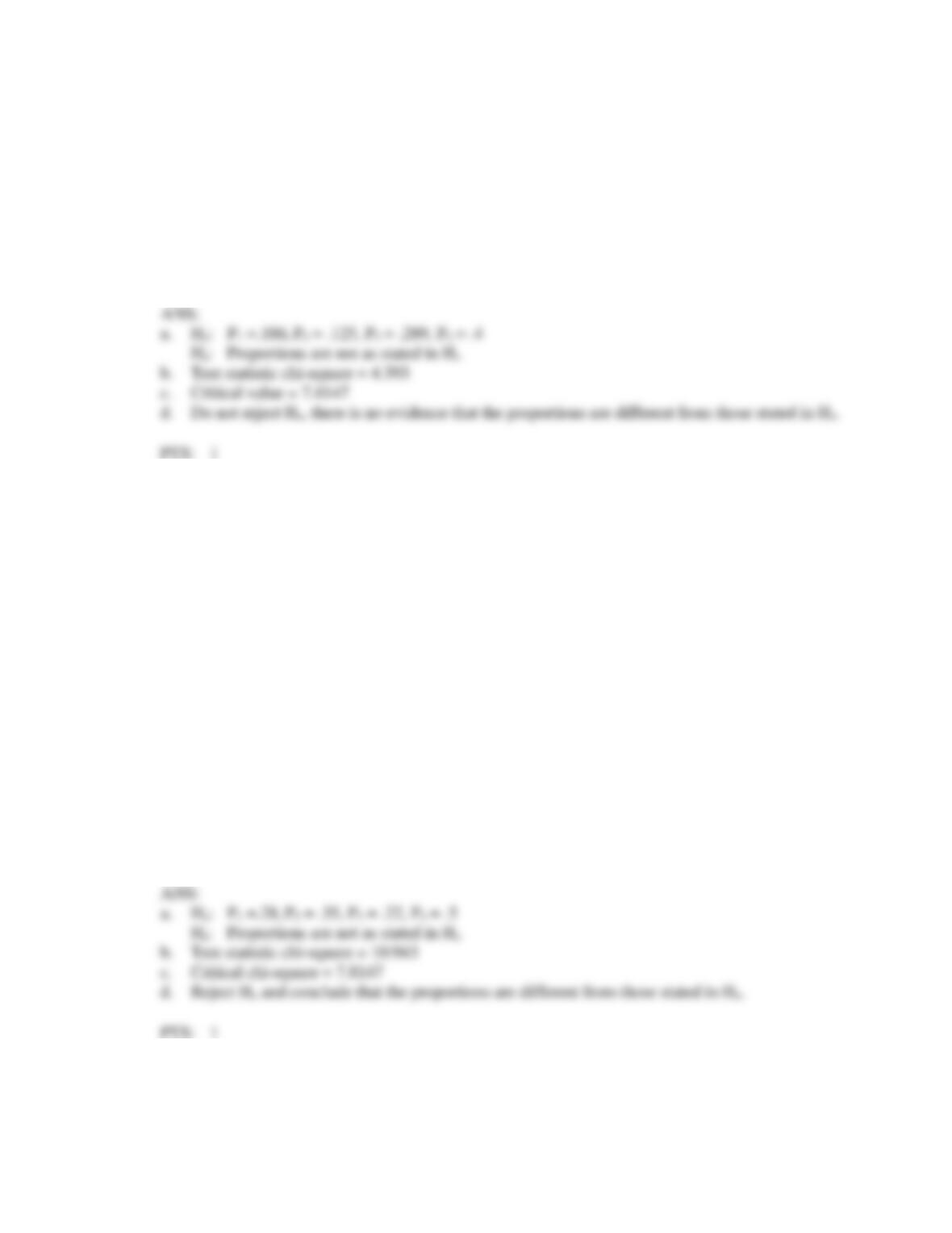
a.
b.
Test statistic chi-square = 10.943
c.
Critical chi-square = 7.8147
d.
Reject Ho and conclude that the proportions are different from those stated in Ho.
30. Before the start of the Winter Olympics, it was expected that the percentages of medals awarded to the
top contenders to be as follows.
a.
b.
Test statistic chi-square = 4.393
c.
Critical value = 7.8147
d.
Do not reject Ho, there is no evidence that the proportions are different from those stated in Ho.
Percentages
United States
25%
Germany
22%
Norway
18%
Austria
14%
Russia
11%
France
10%
Midway through the Olympics, of the 120 medals awarded, the following distribution was observed.
Number of Medals
United States
33
Germany
36
Norway
18
Austria
15
Russia
12
France
6
We want to test to see if there is a significant difference between the expected and actual awards given.
a.
Compute the test statistic.
b.
Using the p-value approach, test to see if there is a significant difference between the expected
and the actual values. Let = .05.
c.
At 95% confidence, test for a significant difference using the critical value approach.
b.