
Exhibit 8-3
A random sample of 81 automobiles traveling on a section of an interstate showed an
average speed of 60 mph. The distribution of speeds of all cars on this section of
highway is normally distributed, with a standard deviation of 13.5 mph.
Refer to Exhibit 8-3. If we are interested in determining an interval estimate for
at
86.9% confidence, the z value to use is
a. 1.96
b. 1.31
c. 1.51
d. 2.00
There are 6 children in a family. The number of children defines a population. The
number of simple random samples of size 2 (without replacement) which are possible
equals
a. 12
b. 15
c. 3
d. 16
For a standard normal distribution, the probability of obtaining a z value between -1.9

to 1.7 is
a. 0.9267
b. 0.4267
c. 1.4267
d. 0.5000
A parameter of the exponential smoothing model which provides the weight given to
the most recent time series value in the calculation of the forecast value is known as the
a. mean square error
b. mean absolute deviation
c. smoothing constant
d. None of these alternatives is correct.
A(n) __________ is a graph of a cumulative distribution.
a. histogram
b. pie chart
c. stem-and-leaf display
d. ogive

Exhibit 12-4
In the past, 35% of the students at ABC University were in the Business College, 35%
of the students were in the Liberal Arts College, and 30% of the students were in the
Education College. To see whether or not the proportions have changed, a sample of
300 students was taken. Ninety of the sample students are in the Business College, 120
are in the Liberal Arts College, and 90 are in the Education College.
Refer to Exhibit 12-4. The expected frequency for the Business College is
a. 0.3
b. 0.35
c. 90
d. 105
A sample of 66 observations will be taken from a process (an infinite population). The
population proportion equals 0.12. The probability that the sample proportion will be
less than 0.1768 is
a. 0.0568
b. 0.0778
c. 0.4222
d. 0.9222

Exhibit 18-5
Forty-one individuals from a sample of 60 indicated they oppose legalized abortion. We
are interested in determining whether or not there is a significant difference between the
proportions of opponents and proponents of legalized abortion.
Refer to Exhibit 18-5. in this problem is
a. 15
b. 5.47
c. 3.87
d. 7.45
A(n) __________ is an unusually small or unusually large data value.
a. sample statistic
b. median
c. z-score
d. outlier
Exhibit 11-5
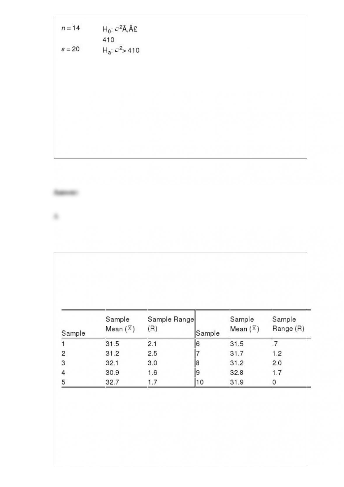
Refer to Exhibit 11-5. The null hypothesis is to be tested at the 5% level of significance.
The critical value(s) from the table is(are)
a. 22.3621
b. 23.6848
c. 5.00874 and 24.7356
d. 5.62872 and 26.119
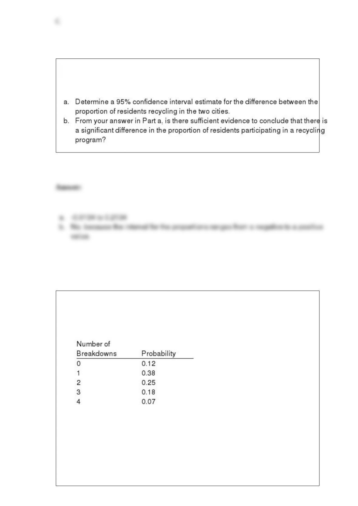
The No-Cal Bottling Company bottles soft drinks for sale to government commissaries.
The bottles come in only one flavor (chocolate-lemon) and only one size (32 ounces).
Joan Stickler, the quality control officer for the commissaries, wants to keep track of the
fill weights of No-Cal and begins to draw daily samples of 100 bottles from the daily
receipts. The first ten sample means and ranges are:
If sample ranges ordinarily average 2.5 ounces:
a. Compute 3s control limits for sample means.
b. Compute 3s control limits for sample ranges.
c. What would you conclude about the fill weights of NoCal?

The sampling distribution for a goodness of fit test is
a. the Poisson distribution
b. the t distribution
c. the normal distribution
d. the chi-square distribution
A tabular representation of the payoffs for a decision problem is a
a. decision tree
b. payoff table
c. matrix
d. sequential matrix

Exhibit 6-5
The weight of items produced by a machine is normally distributed with a mean of 8
ounces and a standard deviation of 2 ounces.
Refer to Exhibit 6-5. What is the random variable in this experiment?
a. the weight of items produced by a machine
b. 8 ounces
c. 2 ounces
d. the normal distribution
Excel’s HYPGEOM.DIST function can be used to compute
a. bin width for histograms
b. hypergeometric probabilities
c. cumulative hypergeometric probabilities
d. Both hypergeometric probabilities and cumulative hypergeometric probabilities are
correct.

Exhibit 5-11
The random variable x is the number of occurrences of an event over an interval of ten
minutes. It can be assumed that the probability of an occurrence is the same in any two
time periods of an equal length. It is known that the mean number of occurrences in ten
minutes is 5.3.
Refer to Exhibit 5-11. The random variable x satisfies which of the following
probability distributions?
a. normal
b. Poisson
c. binomial
d. Not enough information is given to answer this question.
Exhibit 21-2
A simple random sample of 43 elements has been selected from a population of size
800. The sample mean is 500, and the sample standard deviation is 60.
Refer to Exhibit 21-2. The population total is
a. 34,400
b. 21,500
c. 400,000
d. 500,000
Of 150 Chattanooga residents surveyed, 60 indicated that they participated in a
recycling program. In Knoxville, 120 residents were surveyed and 36 claimed to
recycle.
Exhibit 5-4
A local bottling company has determined the number of machine breakdowns per
month and their respective probabilities as shown below.
Refer to Exhibit 5-4. The probability of at least 3 breakdowns in a month is
a. 0.5
b. 0.10
c. 0.30

d. None of the alternative answers is correct.
The relative frequency of a class is computed by
a. dividing the midpoint of the class by the sample size.
b. dividing the frequency of the class by the midpoint.
c. dividing the sample size by the frequency of the class.
d. dividing the frequency of the class by the sample size.
As the degrees of freedom increase, the t distribution approaches the
a. uniform distribution
b. normal distribution
c. exponential distribution
d. p distribution

The Spearman rank-correlation coefficient is
a. a correlation measure based on the average of data items
b. a correlation measure based on rank-ordered data for two variables
c. a correlation measure based on the median of data items
d. None of these alternatives is correct.
To avoid the problem of not having access to Tables of F distribution with values given
for the lower tail, the numerator of the test statistic should be the one with
a. the larger sample size
b. the smaller sample size
c. the larger sample variance
d. the smaller sample variance
Exhibit 16-1
In a regression analysis involving 25 observations, the following estimated regression
equation was developed.
= 10 – 18x1 + 3x2 + 14x3
Also, the following standard errors and the sum of squares were obtained.
Sb1 = 3 Sb2 = 6 Sb3 = 7
SST = 4,800 SSE = 1,296
Refer to Exhibit 16-1. If we are interested in testing for the significance of the
relationship among the variables (i.e., significance of the model) the critical value of F
at = 0.05 is
a. 2.76
b. 2.78
c. 3.10
d. 3.07
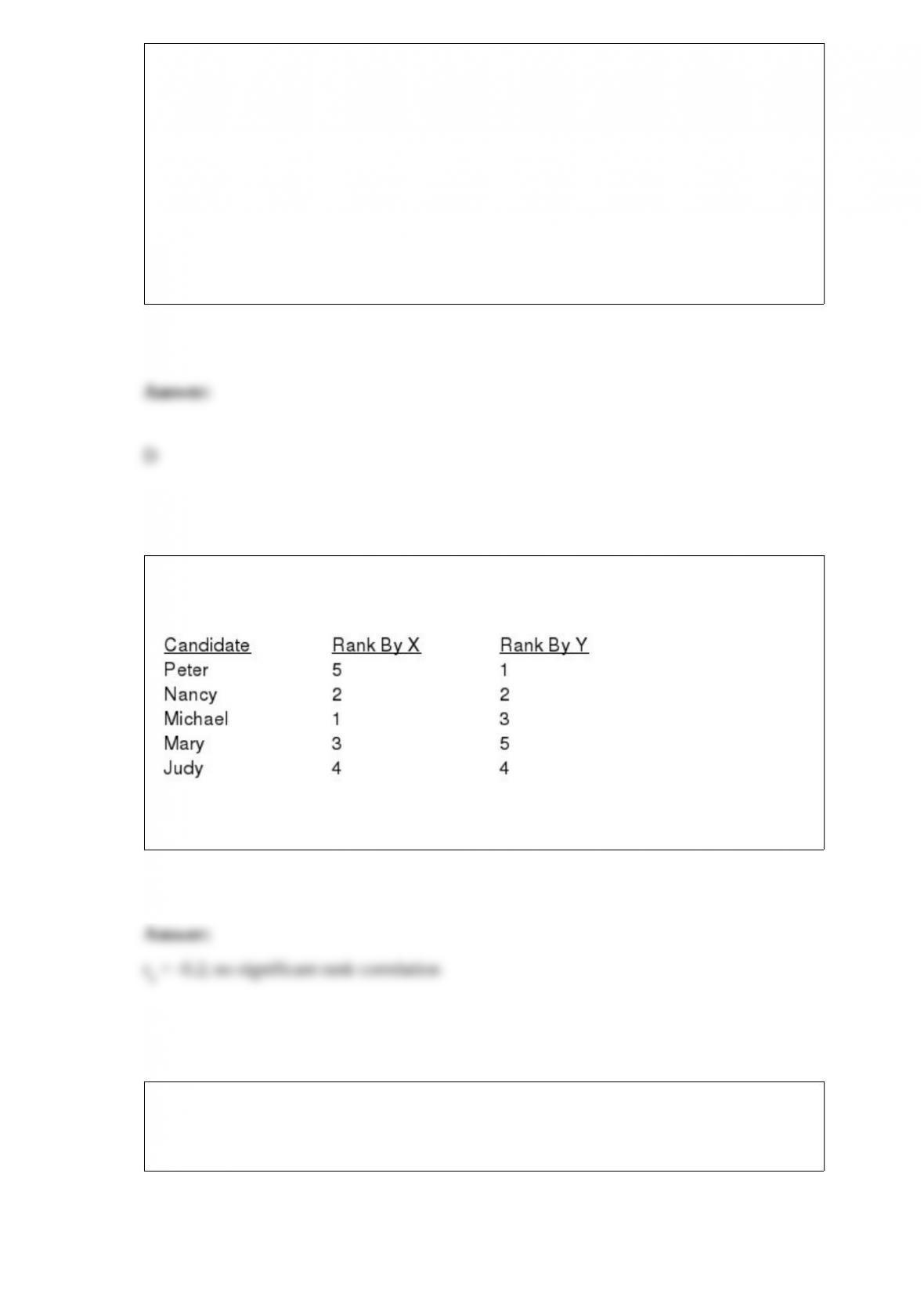
Two faculty members (X and Y) ranked five candidates for scholarships. The rankings
are shown below.
Compute the Spearman rank-correlation and test it for significance. Let = 0.05.
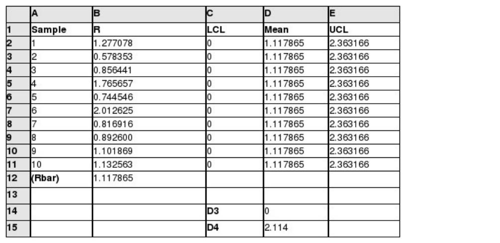
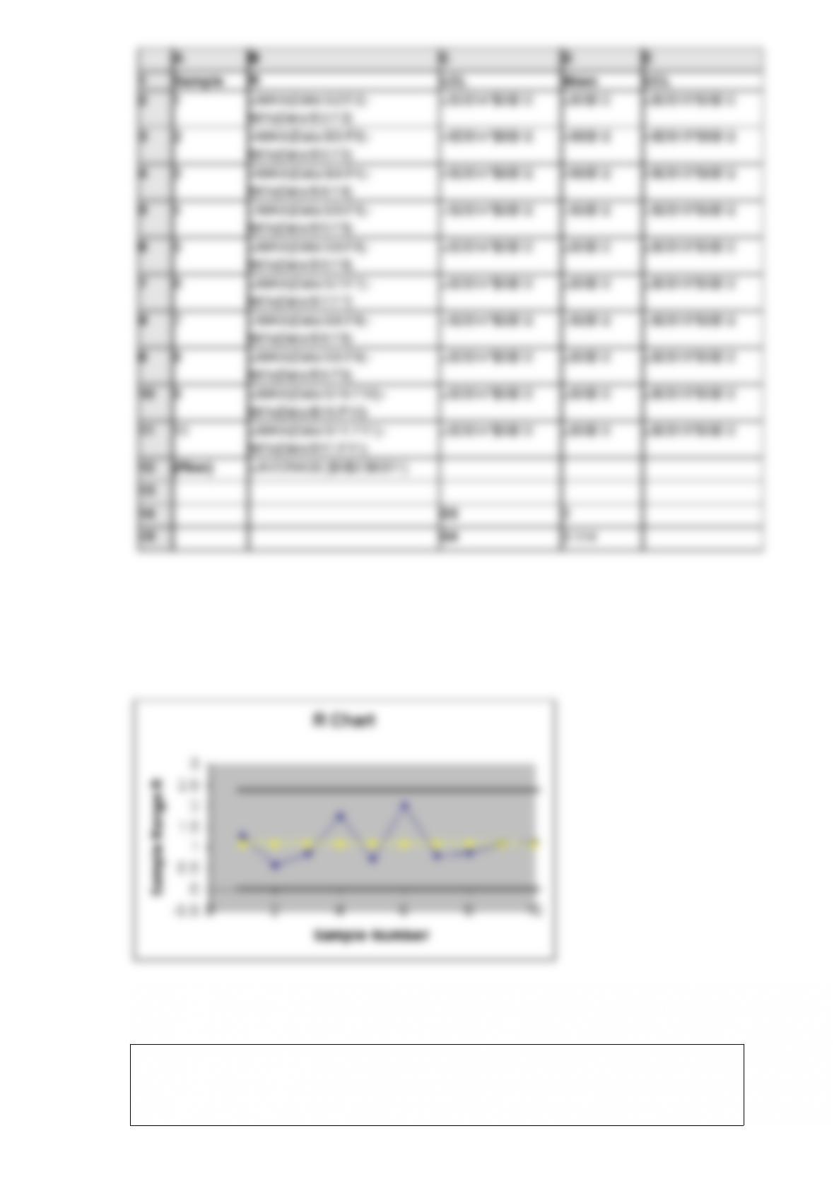
The following data represent the filling weights based on samples of 15 ounce cans of
whole peeled tomatoes. Ten samples of size 5 were taken. Use Excel to develop an R
chart.

Three universities in your state have decided to administer the same comprehensive
examination to the recipients of MBA degrees. From each institution, a random sample
of MBA recipients has been selected and given the test. The following table shows the
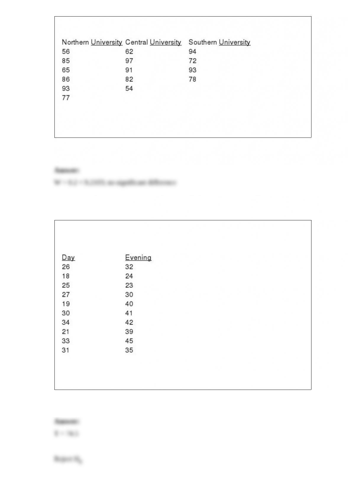
scores of the students from each university.
Use the Kruskal-Wallis test to determine if there is a significant difference in the
average scores of the students from the three universities. Let = 0.01.
Independent random samples of ten day students and ten evening students at a
university showed the following age distributions.
Use = 0.05 and test for any significant differences in the age distribution of the two
populations.
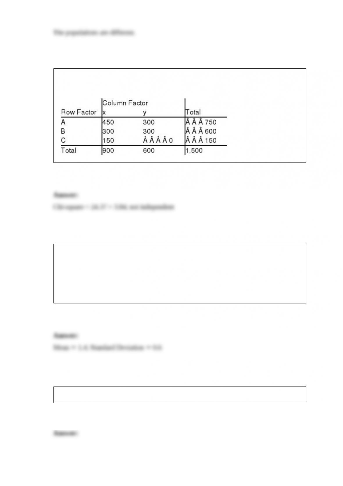
Shown below is a 3 2 contingency table with observed values from a sample of
1,500. At 95% confidence, test for independence of the row and column factors.
The Globe Fishery packs shrimp that weigh more than 1.91 ounces each in packages
marked” large” and shrimp that weigh less than 0.47 ounces each into packages marked
‘small”; the remainder are packed in “medium” size packages. If a day’s catch showed
that 19.77% of the shrimp were large and 6.06% were small, determine the mean and
the standard deviation for the shrimp weights. Assume that the shrimps’ weights are
normally distributed.

The proprietor of a boutique in New York wanted to determine the average age of his
customers. A random sample of 25 customers revealed an average age of 28 years with
a standard deviation of 10 years. Determine a 95% confidence interval estimate for the
average age of all his customers. Assume the population of customer ages is normally
distributed.