Unlock document.
This document is partially blurred.
Unlock all pages and 1 million more documents.
Get Access
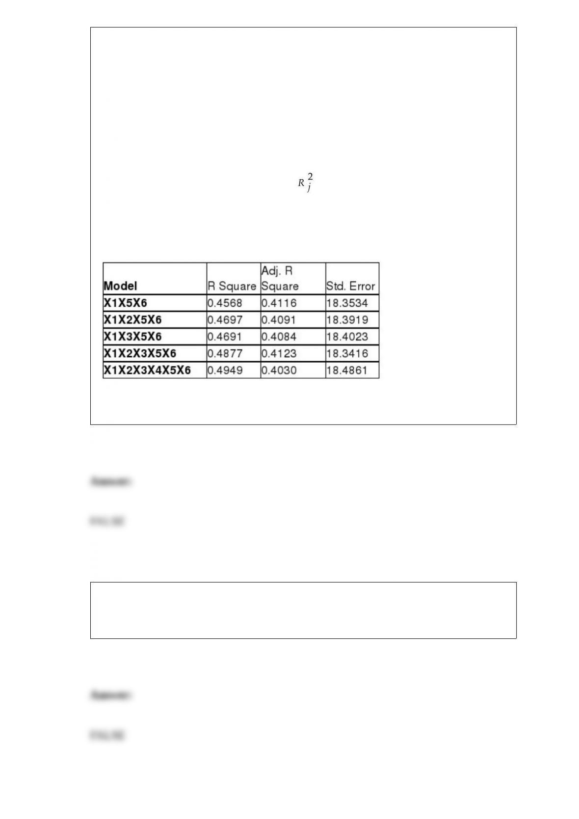
TABLE 15-6
Given below are results from the regression analysis on 40 observations where the
dependent variable is the number of weeks a worker is unemployed due to a layoff (Y)
and the independent variables are the age of the worker (X1), the number of years of
education received (X2), the number of years at the previous job (X3), a dummy variable
for marital status (X4: 1 = married, 0 = otherwise), a dummy variable for head of
household (X5: 1 = yes, 0 = no) and a dummy variable for management position (X6: 1
= yes, 0 = no).
The coefficient of multiple determination ( ) for the regression model using each of
the 6 variables Xj as the dependent variable and all other X variables as independent
variables are, respectively, 0.2628, 0.1240, 0.2404, 0.3510, 0.3342 and 0.0993.
The partial results from best-subset regression are given below:
True or False: Referring to Table 15-6, the variable X4 should be dropped to remove
collinearity.
True or False: If the amount of gasoline purchased per car at a large service station has
a population mean of 15 gallons and a population standard deviation of 4 gallons, then
99.73% of all cars will purchase between 3 and 27 gallons.
True or False: The Paasche price index reflects more accurately the consumption cost at
a point in time because it uses the consumption quantities in the initial year as the base.
True or False: TABLE 17-8
The superintendent of a school district wanted to predict the percentage of students
passing a sixth-grade proficiency test. She obtained the data on percentage of students
passing the proficiency test (% Passing), daily mean of the percentage of students
attending class (% Attendance), mean teacher salary in dollars (Salaries), and
instructional spending per pupil in dollars (Spending) of 47 schools in the state.
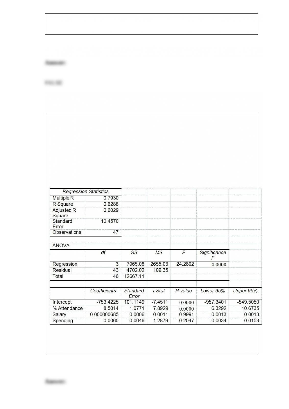
Following is the multiple regression output with Y = % Passing as the dependent
variable, X1 = % Attendance, X2 = Salaries and X3 = Spending:
Referring to Table 17-8, the alternative hypothesis H1 : At least one of βj ≠0 for j =
1, 2, 3 implies that the percentage of students passing the proficiency test is related to
all of the explanatory variables.

True or False: In a particular model, the sum of the squared residuals was 847. If the
model had 5 independent variables, and the data set contained 40 points, the value of
the standard error of the estimate is 24.911.
True or False: Measurement error will become an ethical issue when the findings are
presented without reference to sample size and margin of error.
TABLE 14-15
The superintendent of a school district wanted to predict the
percentage of students passing a sixth-grade proficiency test. She
obtained the data on percentage of students passing the proficiency
test (% Passing), mean teacher salary in thousands of dollars
(Salaries), and instructional spending per pupil in thousands of dollars
(Spending) of 47 schools in the state.
Following is the multiple regression output with Y = % Passing as the
dependent variable, X1 = Salaries and X2 = Spending:

True or False: Referring to Table 14-15, you can conclude definitively
that instructional spending per pupil individually has no impact on the
mean percentage of students passing the proficiency test, taking into
account the e.ect of mean teacher salary, at a 1% level of
significance based solely on but not actually computing the 99% the
confidence interval estimate for β2.
True or False: Referring to Table 14-8, the F test for the significance of the entire
regression performed at a level of significance of 0.01 leads to a rejection of the null
hypothesis.

True or False: Given a data set with 15 yearly observations, there are only seven 9-year
moving averages.
TABLE 9-3
An appliance manufacturer claims to have developed a compact microwave oven that
consumes a mean of no more than 250 W. From previous studies, it is believed that
power consumption for microwave ovens is normally distributed with a population
standard deviation of 15 W. A consumer group has decided to try to discover if the
claim appears true. They take a sample of 20 microwave ovens and find that they
consume a mean of 257.3 W.
True or False: Referring to Table 9-3, the consumer group can conclude that there is
enough evidence that the manufacturer's claim is not true when allowing for a 5%
probability of committing a Type I error.
True or False: In conducting research, you should document both good and bad results.
True or False: A population is the totality of items or things under consideration.
TABLE 15-4
The superintendent of a school district wanted to predict the percentage of students
passing a sixth-grade proficiency test. She obtained the data on percentage of students
passing the proficiency test (% Passing), daily mean of the percentage of students
attending class (% Attendance), mean teacher salary in dollars (Salaries), and
instructional spending per pupil in dollars (Spending) of 47 schools in the state.
Let Y = % Passing as the dependent variable, X1 = % Attendance, X2 = Salaries and X3
= Spending.
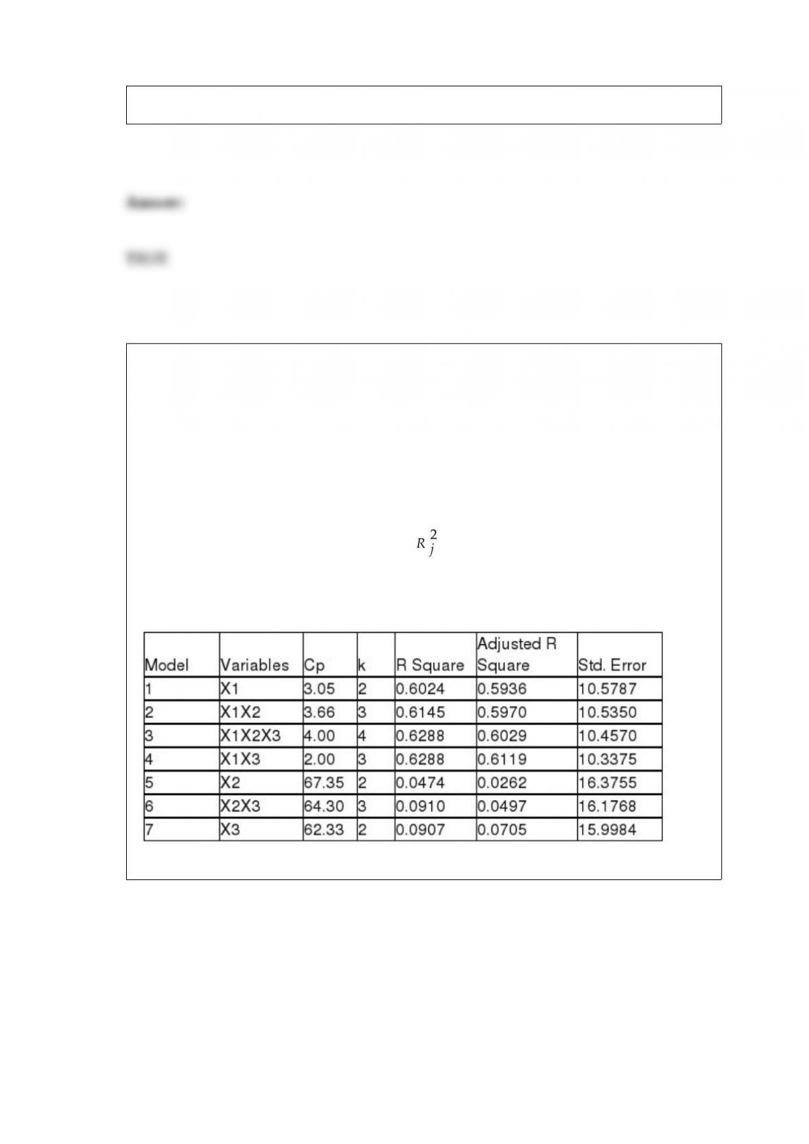
The coefficient of multiple determination ( ) of each of the 3 predictors with all the
other remaining predictors are, respectively, 0.0338, 0.4669, and 0.4743.
The output from the best-subset regressions is given below:
Following is the residual plot for % Attendance:
Following is the output of several multiple regression models:
Model (I):
Model (II):
Model (III):
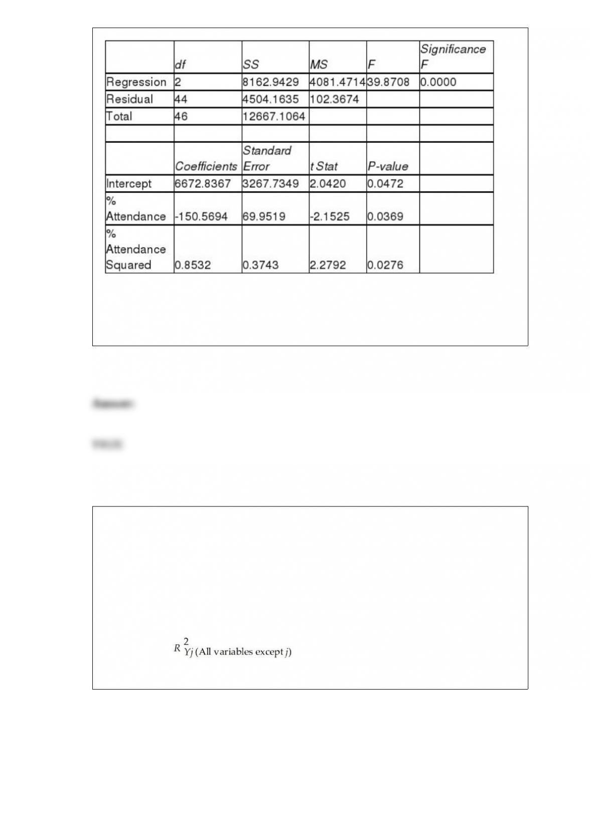
True or False: Referring to Table 15-4, the null hypothesis should be rejected when
testing whether the quadratic effect of daily average of the percentage of students
attending class on percentage of students passing the proficiency test is significant at a
5% level of significance.
True or False: TABLE 17-10
Given below are results from the regression analysis where the dependent variable is
the number of weeks a worker is unemployed due to a layoff (Unemploy) and the
independent variables are the age of the worker (Age), the number of years of education
received (Edu), the number of years at the previous job (Job Yr), a dummy variable for
marital status (Married: 1 = married, 0 = otherwise), a dummy variable for head of
household (Head: 1 = yes, 0 = no) and a dummy variable for management position
(Manager: 1 = yes, 0 = no). We shall call this Model 1. The coefficient of partial
determination ( ) of each of the 6 predictors are, respectively,
0.2807, 0.0386, 0.0317, 0.0141, 0.0958, and 0.1201.
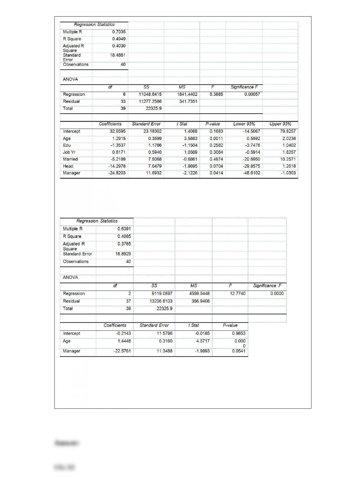
Model 2 is the regression analysis where the dependent variable is Unemploy and the
independent variables are Age and Manager. The results of the regression analysis are
given below:
Referring to Table 17-10, Model 1, we can conclude that, holding constant the effect of
the other independent variables, there is a difference in the mean number of weeks a
worker is unemployed due to a layoff between a worker who is married and one who is
not at a 10% level of significance if we use only the information of the 95% confidence
interval estimate forβ4.

True or False: In general, grouped frequency distributions should have between 5 and
15 class intervals.
An economist is interested to see how consumption for an economy (in $ billions) is
influenced by gross domestic product ($ billions) and aggregate price (consumer price
index). Annual data from 30 years were collected. Which of the following would be the
most appropriate analysis to perform?
A) Simple linear regression
B) Multiple linear regression
C) Exponential smoothing
D) Autoregressive modeling for trend fitting and forecasting
A lab orders 100 rats a week for each of the 52 weeks in the year for experiments that
the lab conducts. Prices for 100 rats follow the following distribution:
How much should the lab budget for next year's rat orders be, assuming this distribution
does not change?
A) $520
B) $637
C) $650
D) $780
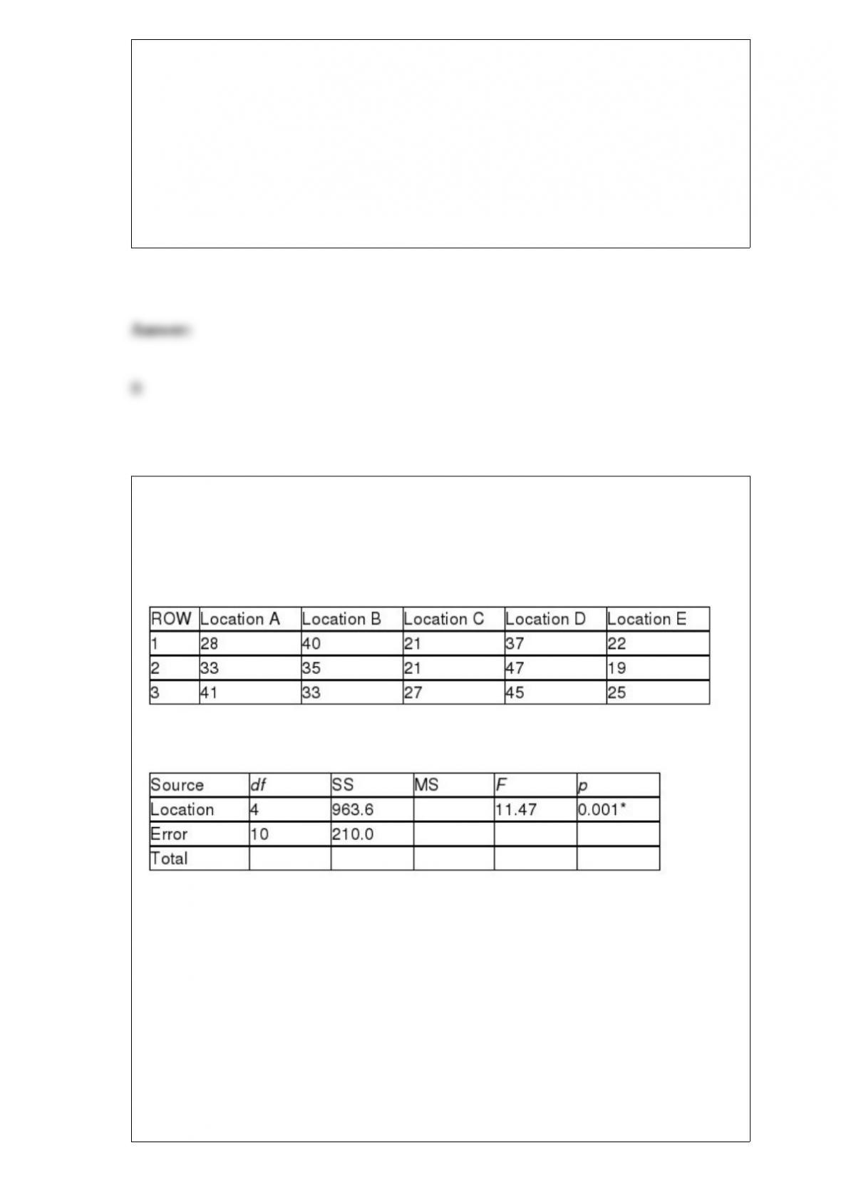
TABLE 11-5
A hotel chain has identically small sized resorts in 5 locations in different small islands.
The data that follow resulted from analyzing the hotel occupancies on randomly
selected days in the 5 locations.
Analysis of Variance
* or p < 0.005, tabular value
Referring to Table 11-5, what should be the decision for the Levene's test for
homogeneity of variances at a 5% level of significance?
A) Reject the null hypothesis because the p-value is smaller than the level of
significance.
B) Reject the null hypothesis because the p-value is larger than the level of significance.
C) Do not reject the null hypothesis because the p-value is smaller than the level of

significance.
D) Do not reject the null hypothesis because the p-value is larger than the level of
significance.
TABLE 17-9
What are the factors that determine the acceleration time (in sec.) from 0 to 60 miles per
hour of a car? Data on the following variables for 171 different vehicle models were
collected:
Accel Time: Acceleration time in sec.
Cargo Vol: Cargo volume in cu. ft.
HP: Horsepower
MPG: Miles per gallon
SUV: 1 if the vehicle model is an SUV with Coupe as the base when SUV and Sedan
are both 0
Sedan: 1 if the vehicle model is a sedan with Coupe as the base when SUV and Sedan
are both 0
The regression results using acceleration time as the dependent variable and the
remaining variables as the independent variables are presented below.
The various residual plots are as shown below.
The coefficient of partial determination ( ) of each of the 5
predictors are, respectively, 0.0380, 0.4376, 0.0248, 0.0188, and 0.0312.

The coefficient of multiple determination for the regression model using each of the 5
variables Xj as the dependent variable and all other X variables as independent variables
( ) are, respectively, 0.7461, 0.5676, 0.6764, 0.8582, 0.6632.
Referring to Table 17-9, which of the following assumptions is most likely violated
based on the residual plot of the residuals versus predicted Y?
A) Independence of errors
B) Normality of errors
C) Equal variance
D) None of the above
TABLE 17-6
A weight-loss clinic wants to use regression analysis to build a model for weight loss of
a client (measured in pounds). Two variables thought to affect weight loss are client's
length of time on the weight-loss program and time of session. These variables are
described below:
Y = Weight loss (in pounds)
X1 = Length of time in weight-loss program (in months)
X2 = 1 if morning session, 0 if not
X3 = 1 if afternoon session, 0 if not (Base level = evening session)
Data for 12 clients on a weight-loss program at the clinic were collected and used to fit
the interaction model:
Y = β0 + β1X1 + β2X2 + β3X3 + β4X1X2 + β5X1X3 + ε
Partial output from Microsoft Excel follows:
Regression Statistics
ANOVA
F = 5.41118 Significance F = 0.040201
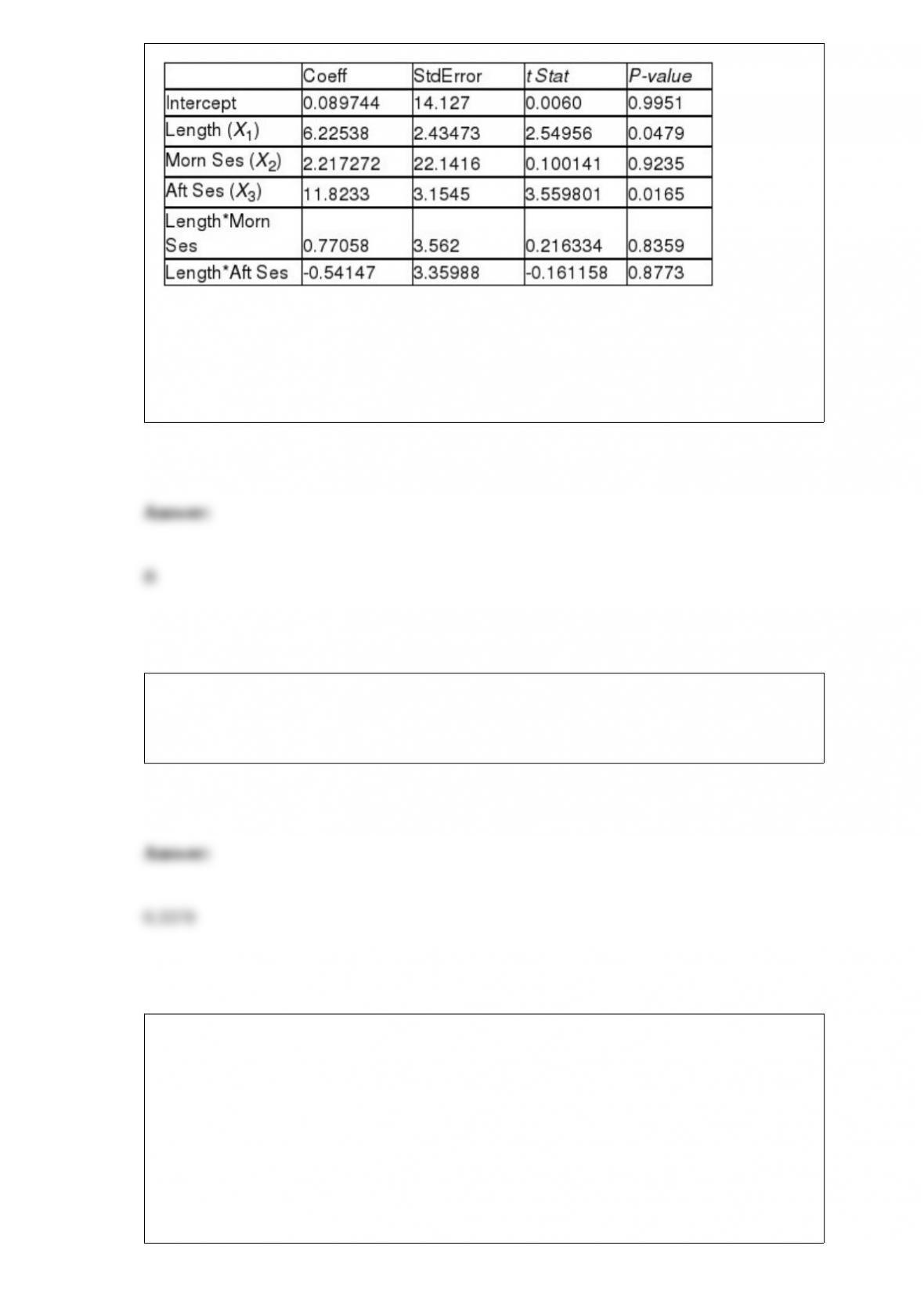
Referring to Table 17-6, what is the experimental unit for this analysis?
A) a clinic
B) a client on a weight-loss program
C) a month
D) a morning, afternoon, or evening session
Suppose that past history shows that 60% of college students prefer Brand C cola. A
sample of 5 students is to be selected. The probability that more than 3 prefer brand C is
________.
Which of the following is most likely a parameter as opposed to a statistic?
A) the average score of the first five students completing an assignment
B) the proportion of females registered to vote in a county
C) the average height of people randomly selected from a database
D) the proportion of trucks stopped yesterday that were cited for bad brakes

Which of the following terms describes the up and down movements of a time series
that vary both in length and intensity?
A) trend
B) cyclical component
C) irregular component
D) seasonal component
Which of the following statements about the sampling distribution of the sample mean
is incorrect?
A) The sampling distribution of the sample mean is approximately normal whenever the
sample size is sufficiently large (n >= 30).
B) The sampling distribution of the sample mean is generated by repeatedly taking
samples of size n and computing the sample means.
C) The mean of the sampling distribution of the sample mean is equal to .
D) The standard deviation of the sampling distribution of the sample mean is equal to
.

The use of the finite population correction factor when sampling without replacement
from finite populations will
A) increase the standard error of the mean.
B) not affect the standard error of the mean.
C) reduce the standard error of the mean.
D) only affect the proportion, not the mean.
TABLE 9-2
A student claims that he can correctly identify whether a person is a business major or
an agriculture major by the way the person dresses. Suppose in actuality that if someone
is a business major, he can correctly identify that person as a business major 87% of the
time. When a person is an agriculture major, the student will incorrectly identify that
person as a business major 16% of the time. Presented with one person and asked to
identify the major of this person (who is either a business or an agriculture major), he
considers this to be a hypothesis test with the null hypothesis being that the person is a
business major and the alternative that the person is an agriculture major.
Referring to Table 9-2, what would be a Type I error?
A) Saying that the person is a business major when in fact the person is a business
major.
B) Saying that the person is a business major when in fact the person is an agriculture
major.
C) Saying that the person is an agriculture major when in fact the person is a business
major.
D) Saying that the person is an agriculture major when in fact the person is an
agriculture major.

A sample of 100 fuses from a very large shipment is found to have 10 that are defective.
Based on this information, which of the following will you construct to learn about the
proportion of fuses that are defective?
A) Confidence interval estimate for the total using the Student's t distribution
B) Confidence interval estimate for the mean using the Student's t distribution
C) Confidence interval estimate for the proportion using the standard normal
distribution
D) Confidence interval estimate for the difference between two means using the
standard normal distribution
The value of the cumulative standardized normal distribution at 1.5X is 0.9332. The
value of X is
A) 0.10.
B) 0.50.
C) 1.00.
D) 1.50.
TABLE 1-2
A Wall Street Journal poll asked 2,150 adults in the United States a series of questions
to find out their view on the U.S. economy.
Referring to Table 1-2, the possible responses to the question "Are you 1. Currently
employed,
2. Unemployed but actively looking for job, 3. Unemployed and quit looking for job?"
are values from a
A) discrete numerical variable.
B) continuous numerical variable.
C) categorical variable.
D) table of random numbers.
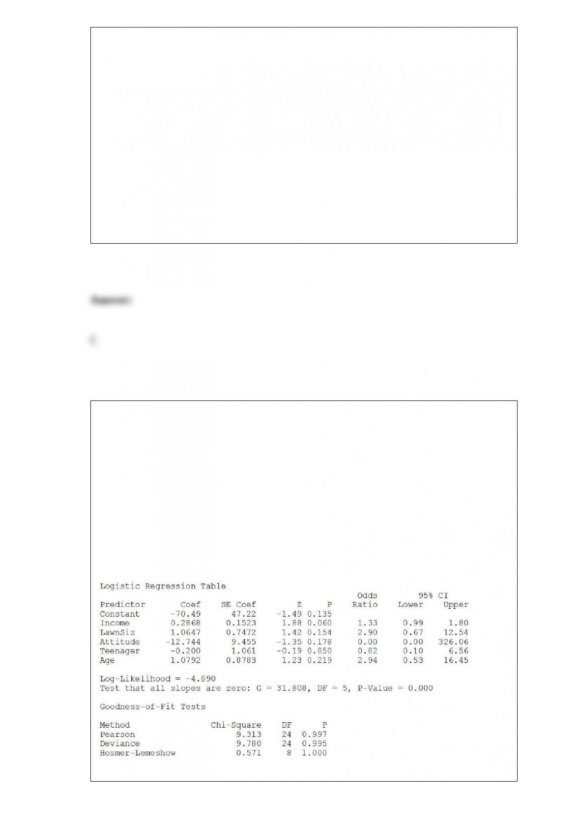
TABLE 17-12
The marketing manager for a nationally franchised lawn service company would like to
study the characteristics that differentiate home owners who do and do not have a lawn
service. A random sample of 30 home owners located in a suburban area near a large
city was selected; 15 did not have a lawn service (code 0) and 15 had a lawn service
(code 1). Additional information available concerning these 30 home owners includes
family income (Income, in thousands of dollars), lawn size (Lawn Size, in thousands of
square feet), attitude toward outdoor recreational activities (Attitude 0 = unfavorable, 1
= favorable), number of teenagers in the household (Teenager), and age of the head of
the household (Age).
The Minitab output is given below:
Referring to Table 17-12, which of the following is the correct interpretation for the

Attitude slope coefficient?
A) Holding constant the effect of the other variables, the estimated number of lawn
services purchased is 12.74 lower for a home owner who has a favorable attitude
toward outdoor recreational activities than one that has an unfavorable attitude.
B) Holding constant the effect of the other variables, the estimated odds ratio of
purchasing a lawn service is 12.74 lower for a home owner who has a favorable attitude
toward outdoor recreational activities than one that has an unfavorable attitude.
C) Holding constant the effect of the other variables, the estimated natural logarithm of
the odds ratio of purchasing a lawn service is 12.74 lower for a home owner who has a
favorable attitude toward outdoor recreational activities than one that has an
unfavorable attitude.
D) Holding constant the effect of the other variables, the estimated probability of
purchasing a lawn service is 12.74 lower for a home owner who has a favorable attitude
toward outdoor recreational activities than one that has an unfavorable attitude.
TABLE 17-8
The superintendent of a school district wanted to predict the percentage of students
passing a sixth-grade proficiency test. She obtained the data on percentage of students
passing the proficiency test (% Passing), daily mean of the percentage of students
attending class (% Attendance), mean teacher salary in dollars (Salaries), and
instructional spending per pupil in dollars (Spending) of 47 schools in the state.
Following is the multiple regression output with Y = % Passing as the dependent
variable, X1 = % Attendance, X2 = Salaries and X3 = Spending:
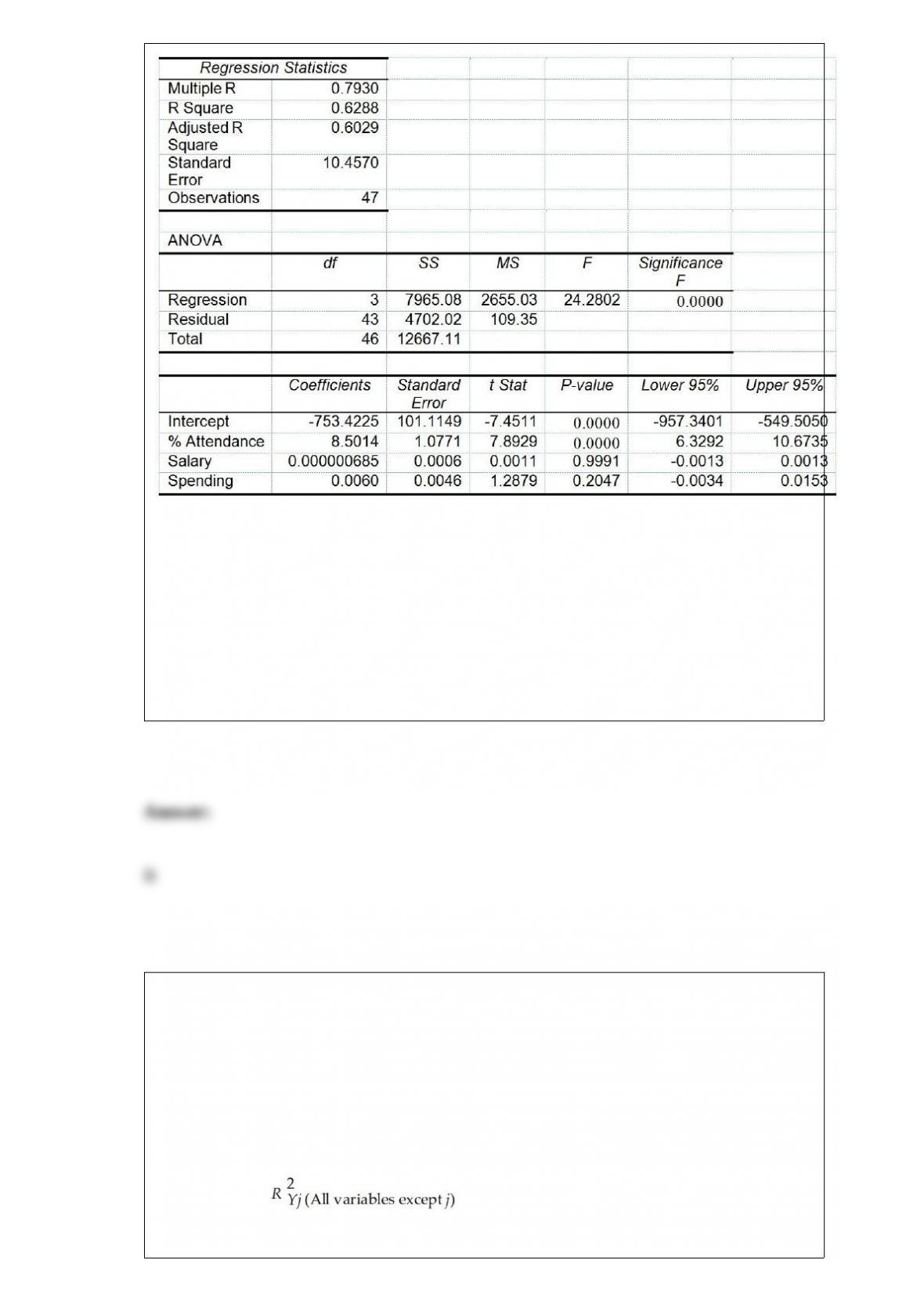
Referring to Table 17-8, which of the following is the correct alternative hypothesis to
test whether the daily mean of the percentage of students attending class has any effect
on the percentage of students passing the proficiency test, taking into account the effect
of all the other independent variables?
A) H1 : β0 ≠0
B) H1 : β1 ≠0
C) H1 : β2 ≠0
D) H1 : β3 ≠0
TABLE 17-10
Given below are results from the regression analysis where the dependent variable is
the number of weeks a worker is unemployed due to a layoff (Unemploy) and the
independent variables are the age of the worker (Age), the number of years of education
received (Edu), the number of years at the previous job (Job Yr), a dummy variable for
marital status (Married: 1 = married, 0 = otherwise), a dummy variable for head of
household (Head: 1 = yes, 0 = no) and a dummy variable for management position
(Manager: 1 = yes, 0 = no). We shall call this Model 1. The coefficient of partial
determination ( ) of each of the 6 predictors are, respectively,
0.2807, 0.0386, 0.0317, 0.0141, 0.0958, and 0.1201.
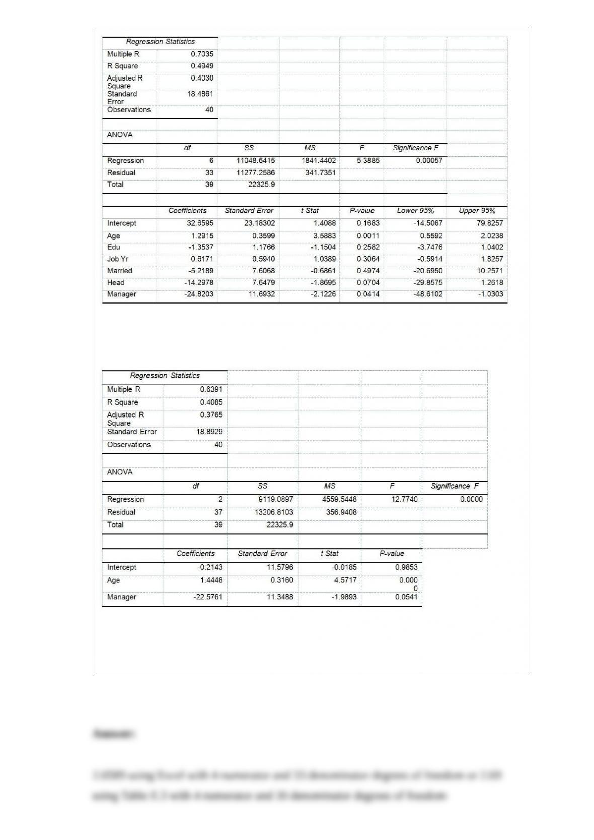
Model 2 is the regression analysis where the dependent variable is Unemploy and the
independent variables are Age and Manager. The results of the regression analysis are
given below:
Referring to Table 17-10 and using both Model 1 and Model 2, what is the critical value
of the test statistic for testing whether the independent variables that are not significant
individually are also not significant as a group in explaining the variation in the
dependent variable at a 5% level of significance?
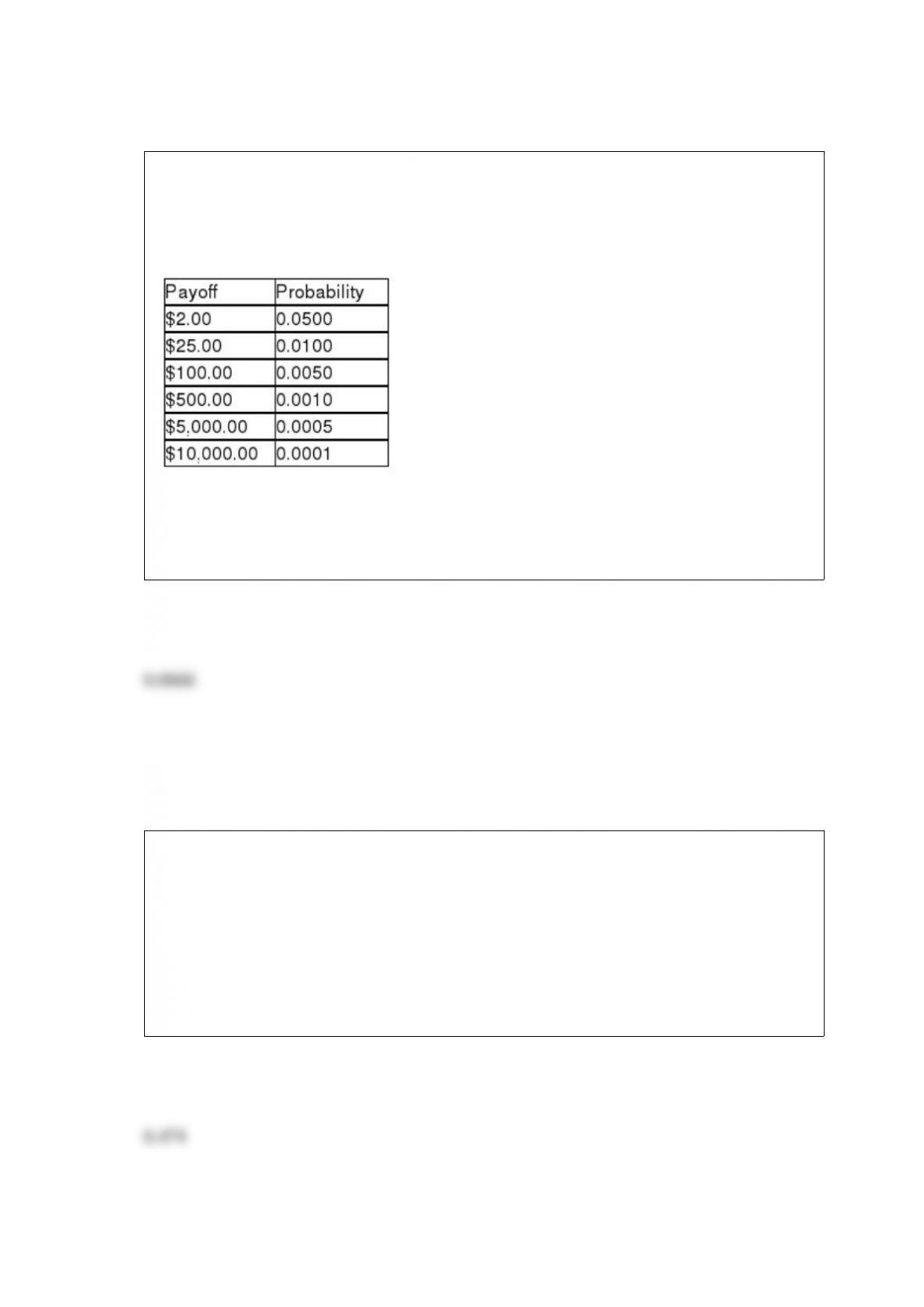
TABLE 4-7
The next state lottery will have the following payoffs possible with their associated
probabilities.
You buy a single ticket.
Referring to Table 4-7, the probability that you win any money is ________.
TABLE 4-8
According to the record of the registrar's office at a state university, 35% of the students
are freshman, 25% are sophomore, 16% are junior and the rest are senior. Among the
freshmen, sophomores, juniors and seniors, the portion of students who live in the
dormitory are, respectively, 80%, 60%, 30% and 20%.
Referring to Table 4-8, what percentage of the students do not live in a dormitory?
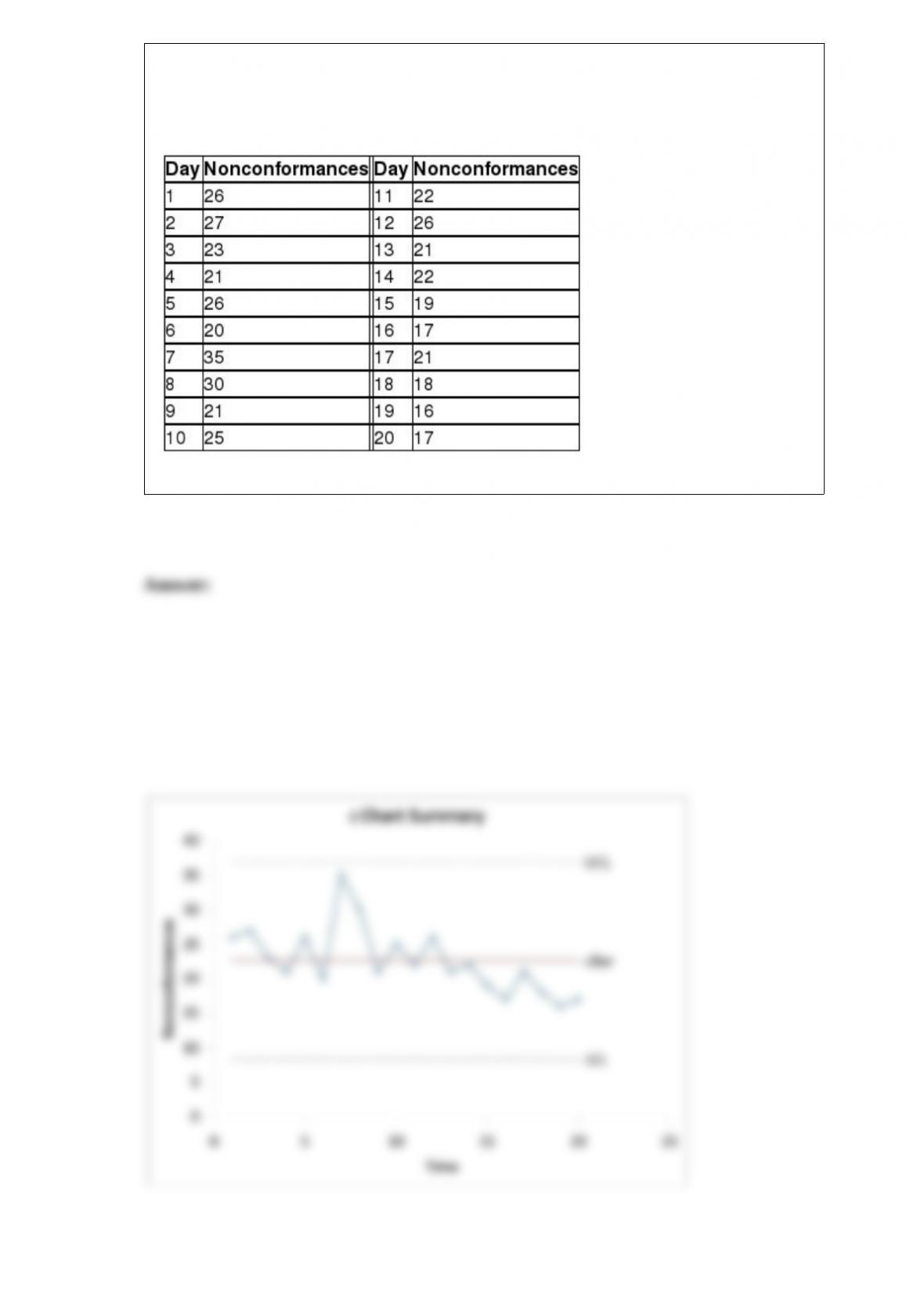
TABLE 18-10
Below is the number of defective items from a production line over twenty consecutive
morning shifts.
Referring to Table 18-10, construct a c chart for the number of defective items.
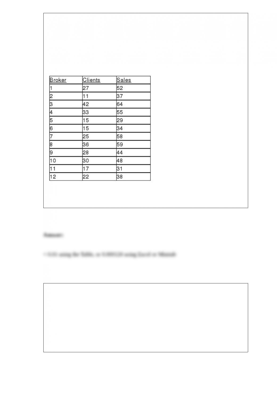
TABLE 13-4
The managers of a brokerage firm are interested in finding out if the number of new
clients a broker brings into the firm affects the sales generated by the broker. They
sample 12 brokers and determine the number of new clients they have enrolled in the
last year and their sales amounts in thousands of dollars. These data are presented in the
table that follows.
Referring to Table 13-4, the managers of the brokerage firm wanted to test the
hypothesis that the population slope was equal to 0. The p-value of the test is ________.
TABLE 9-1
Microsoft Excel was used on a set of data involving the number of defective items
found in a random sample of 46 cases of light bulbs produced during a morning shift at
a plant. A manager wants to know if the mean number of defective bulbs per case is
greater than 20 during the morning shift. She will make her decision using a test with a
level of significance of 0.10. The following information was extracted from the
Microsoft Excel output for the sample of 46 cases:
Referring to Table 9-1, state the alternative hypothesis for this study.
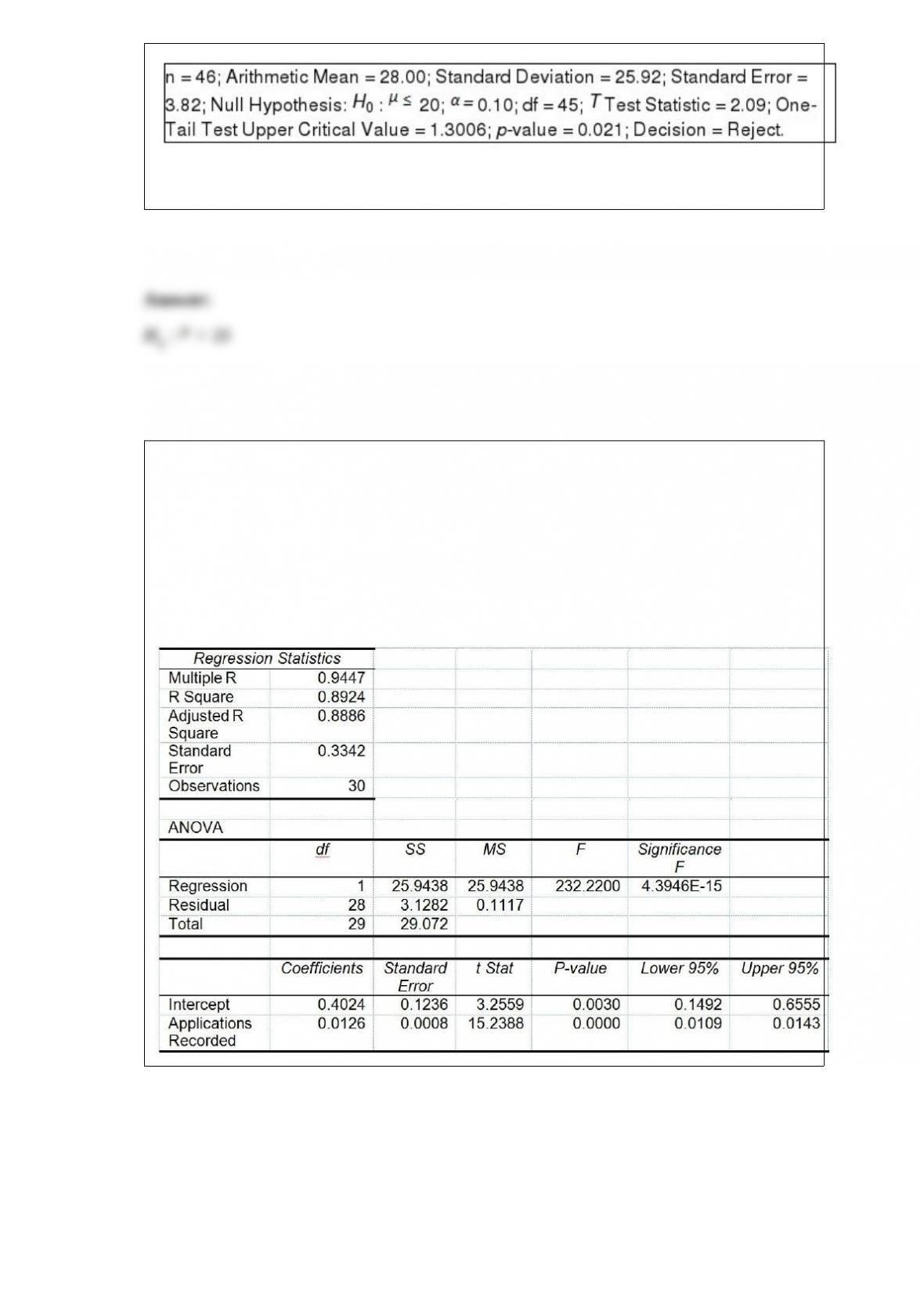
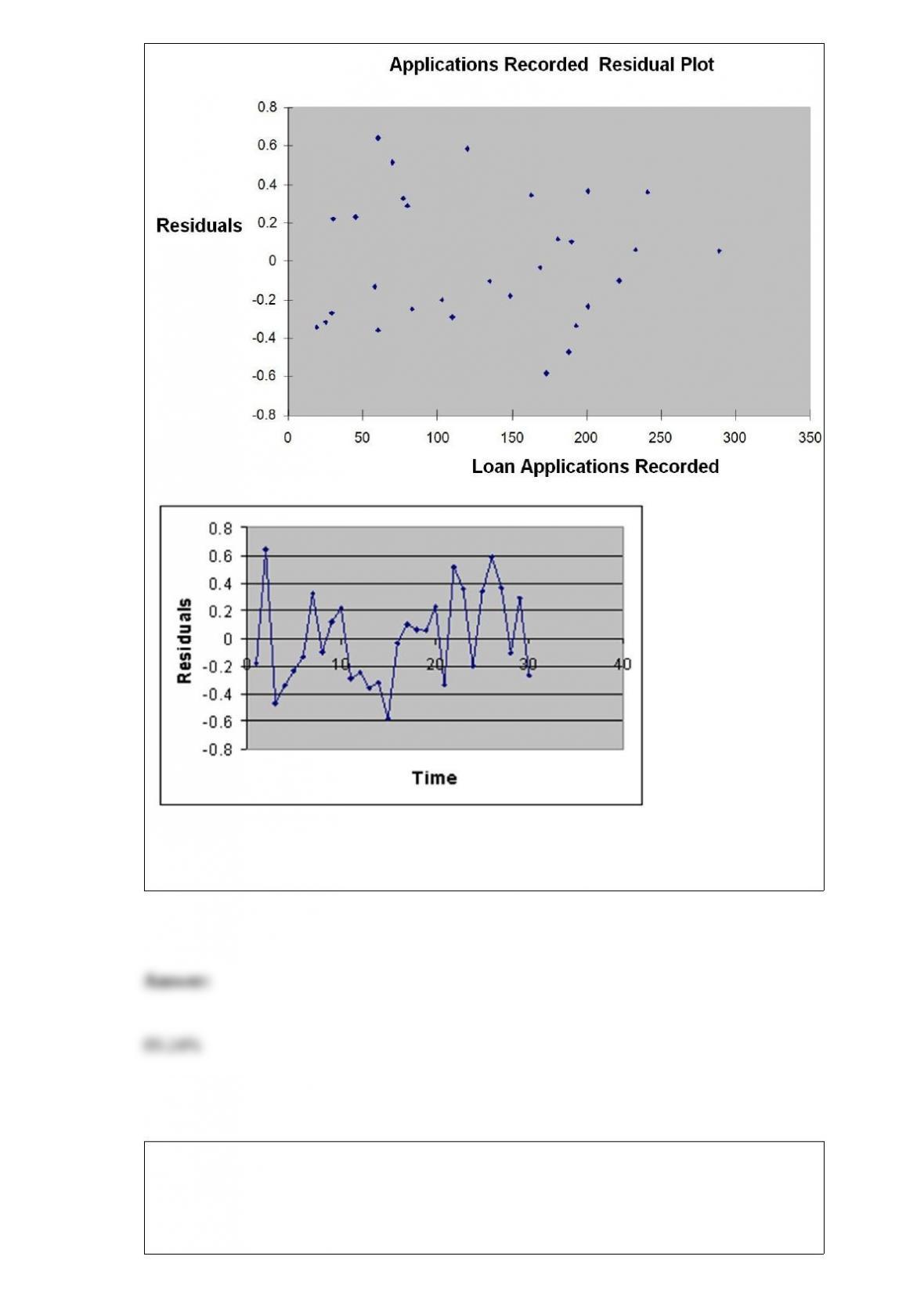
TABLE 13-12
The manager of the purchasing department of a large saving and loan organization
would like to develop a model to predict the amount of time (measured in hours) it
takes to record a loan application. Data are collected from a sample of 30 days, and the
number of applications recorded and completion time in hours is recorded. Below is the
regression output:
Referring to Table 13-12, what percentage of the variation in the amount of time needed
can be explained by the variation in the number of invoices processed?
TABLE 18-9
The manufacturer of canned food constructed control charts and analyzed several
quality characteristics. One characteristic of interest is the weight of the filled cans. The
lower specification limit for weight is 2.95 pounds. The table below provides the range
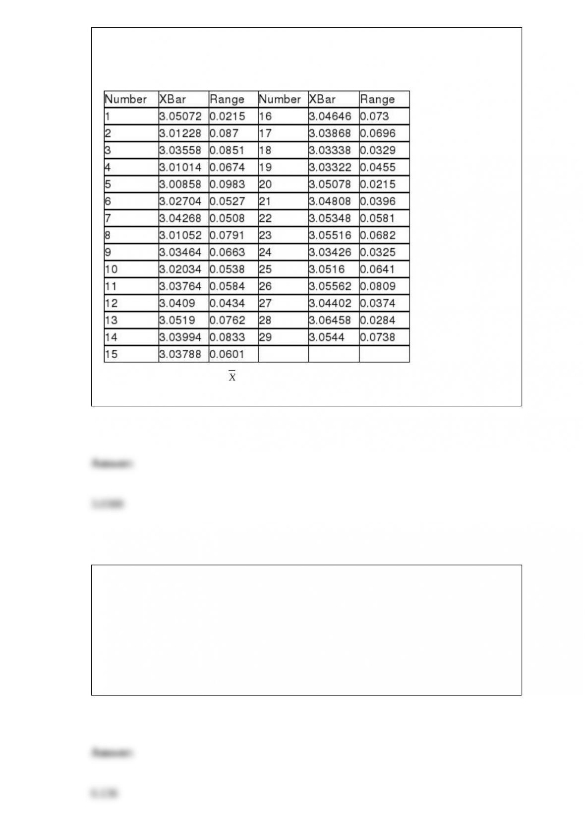
and mean of the weights of five cans tested every fifteen minutes during a day's
production.
Referring to Table 18-9, an chart is to be used for the weight. The center line of this
chart is located at ________.
TABLE 4-6
At a Texas college, 60% of the students are from the southern part of the state, 30% are
from the northern part of the state, and the remaining 10% are from out-of-state. All
students must take and pass an Entry
Referring to Table 4-6, if a randomly selected student has passed the ELM, the
probability that the student is from out-of-state is ________.
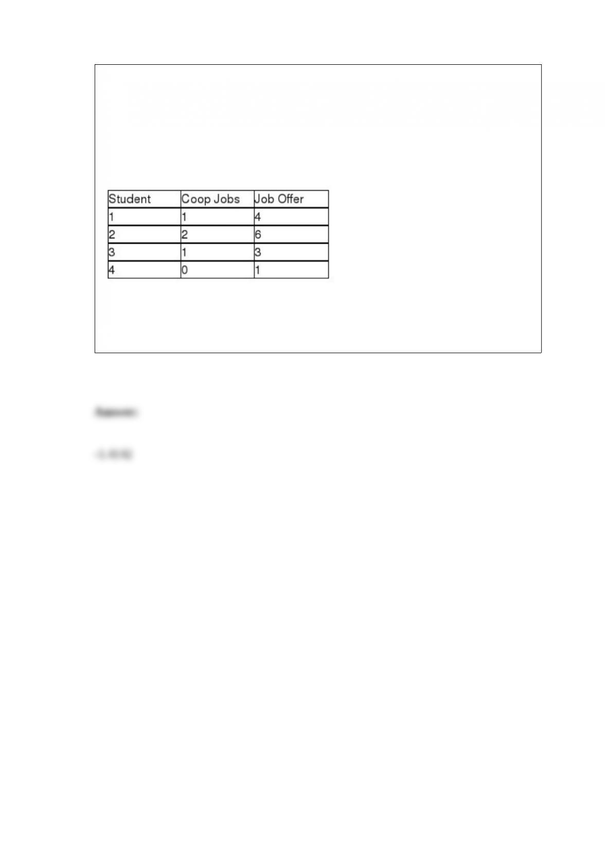
TABLE 13-3
The director of cooperative education at a state college wants to examine the effect of
cooperative education job experience on marketability in the work place. She takes a
random sample of 4 students. For these 4, she finds out how many times each had a
cooperative education job and how many job offers they received upon graduation.
These data are presented in the table below.
Referring to Table 13-3, the director of cooperative education wanted to test the
hypothesis that the population slope was equal to 3.0. The value of the test statistic is
________.


