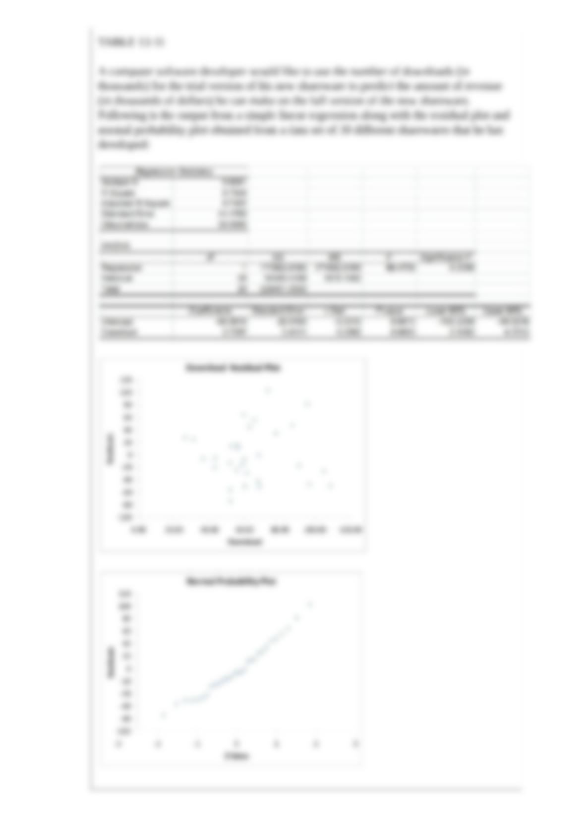
TABLE 13-11
A computer software developer would like to use the number of downloads (in
thousands) for the trial version of his new shareware to predict the amount of revenue
(in thousands of dollars) he can make on the full version of the new shareware.
Following is the output from a simple linear regression along with the residual plot and
normal probability plot obtained from a data set of 30 different sharewares that he has
developed:

True or False: Referring to Table 13-11, the normality of error assumption appears to
have been violated.
True or False: As the size of the sample is increased, the standard deviation of the
sampling distribution of the sample mean for a normally distributed population will stay
the same.
True or False: TABLE 17-8
The superintendent of a school district wanted to predict the percentage of students
passing a sixth-grade proficiency test. She obtained the data on percentage of students
passing the proficiency test (% Passing), daily mean of the percentage of students
attending class (% Attendance), mean teacher salary in dollars (Salaries), and
instructional spending per pupil in dollars (Spending) of 47 schools in the state.
Following is the multiple regression output with Y = % Passing as the dependent
variable, X1 = % Attendance, X2 = Salaries and X3 = Spending:
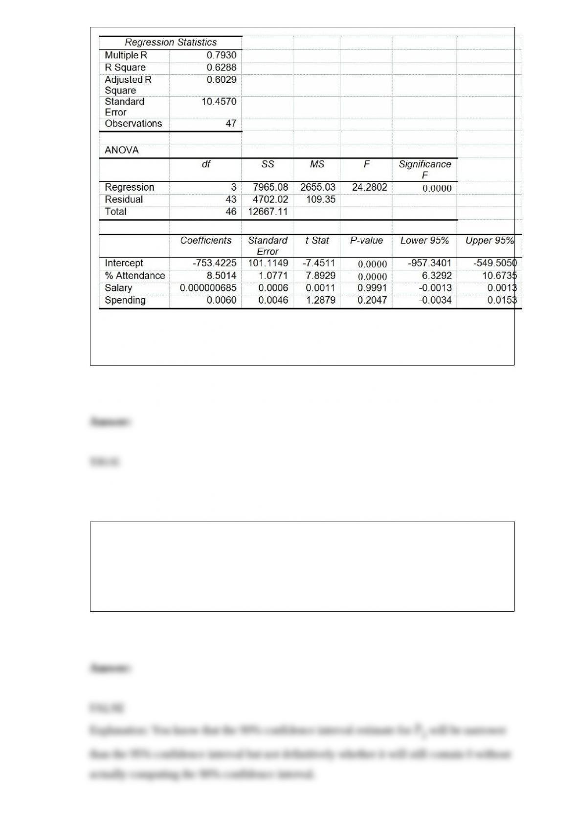
Referring to Table 17-8, the null hypothesis H0 : β1 = β2 = β3 = 0 implies that the
percentage of students passing the proficiency test is not affected by any of the
explanatory variables.
True or False: Referring to Table 14-15, you can conclude definitively that instructional
spending per pupil individually has no impact on the mean percentage of students
passing the proficiency test, taking into account the effect of mean teacher salary, at a
10% level of significance based solely on but not actually computing the 90%
confidence interval estimate for β2.
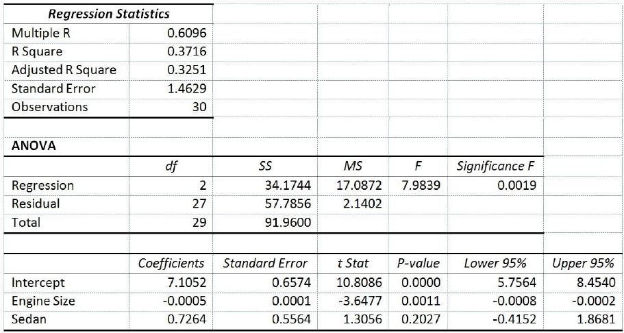
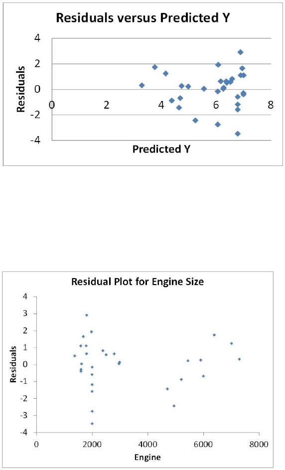
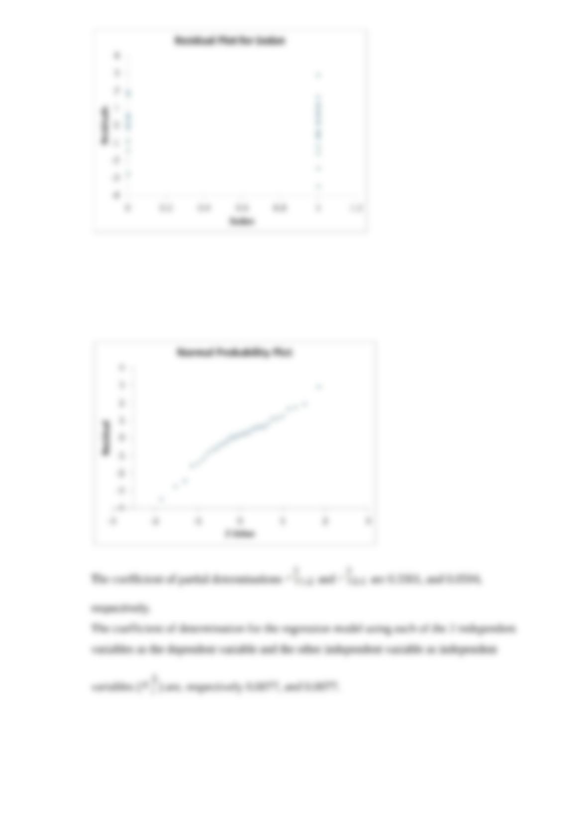

TABLE 14-17
Given below are results from the regression analysis where the
dependent variable is the number of weeks a worker is unemployed
due to a layo! (Unemploy) and the independent variables are the age
of the worker (Age) and a dummy variable for management position
(Manager: 1 = yes, 0 = no).
The results of the regression analysis are given below:
True or False: Referring to Table 14-17, the null hypothesis H0 : β1 =
β2 = 0 implies that the number of weeks a worker is unemployed due
to a layo! is not a!ected by some of the explanatory variables.
TABLE 9-1
Microsoft Excel was used on a set of data involving the number of defective items

found in a random sample of 46 cases of light bulbs produced during a morning shift at
a plant. A manager wants to know if the mean number of defective bulbs per case is
greater than 20 during the morning shift. She will make her decision using a test with a
level of significance of 0.10. The following information was extracted from the
Microsoft Excel output for the sample of 46 cases:
True or False: Referring to Table 9-1, the manager can conclude that there is sufficient
evidence to show that the mean number of defective bulbs per case is greater than 20
during the morning shift using a level of significance of 0.10.
TABLE 8-6
After an extensive advertising campaign, the manager of a company wants to estimate
the proportion of potential customers that recognize a new product. She samples 120
potential consumers and finds that 54 recognize this product. She uses this sample
information to obtain a 95% confidence interval that goes from 0.36 to 0.54.
True or False: Referring to Table 8-6, 95% of the time, the sample proportion of people
that recognize the product will fall between 0.36 and 0.54.
True or False: The Laspeyres price index is a form of weighted aggregate price index.

True or False: In a set of numerical data, the value for Q2 is always halfway between Q1
and Q3.
True or False: TABLE 17-9
What are the factors that determine the acceleration time (in sec.) from 0 to 60 miles per
hour of a car? Data on the following variables for 171 different vehicle models were
collected:
Accel Time: Acceleration time in sec.
Cargo Vol: Cargo volume in cu. ft.
HP: Horsepower
MPG: Miles per gallon
SUV: 1 if the vehicle model is an SUV with Coupe as the base when SUV and Sedan
are both 0
Sedan: 1 if the vehicle model is a sedan with Coupe as the base when SUV and Sedan
are both 0
The regression results using acceleration time as the dependent variable and the
remaining variables as the independent variables are presented below.
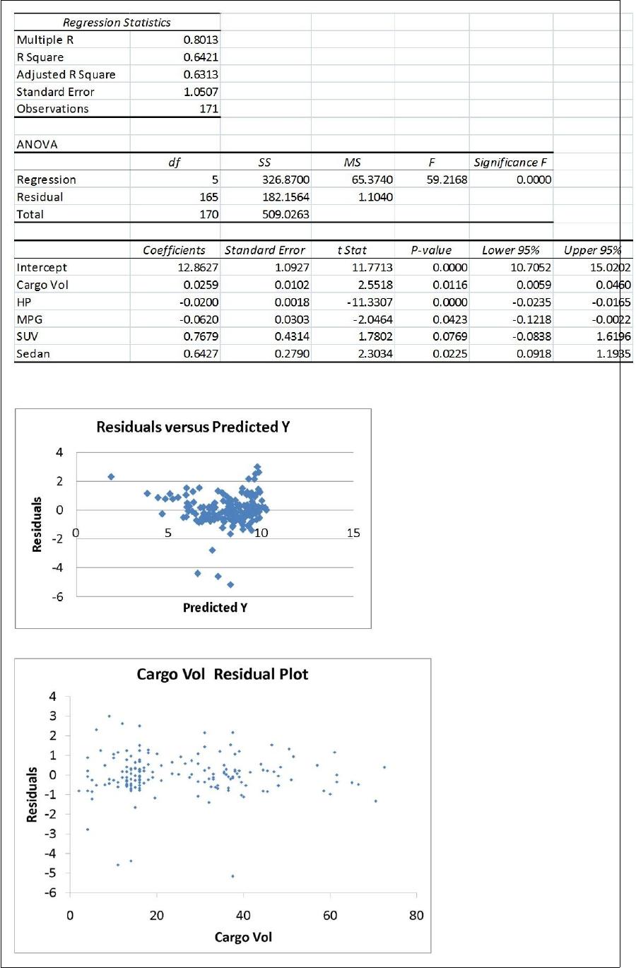
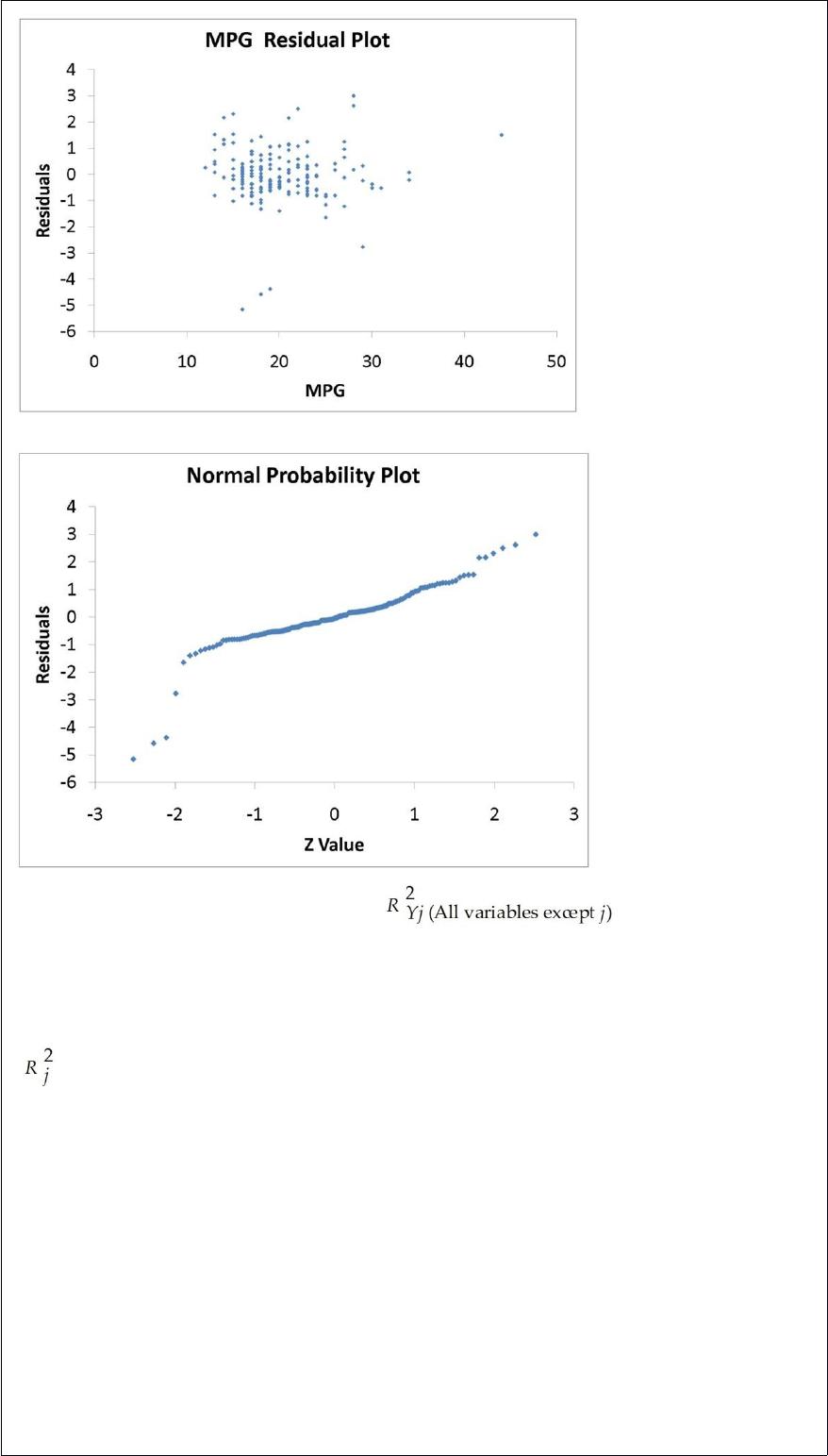
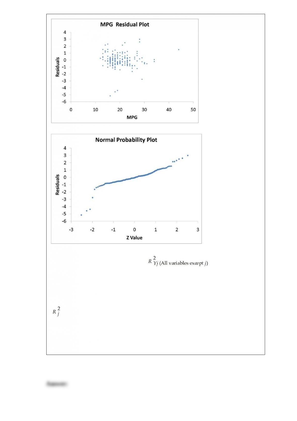
The various residual plots are as shown below.
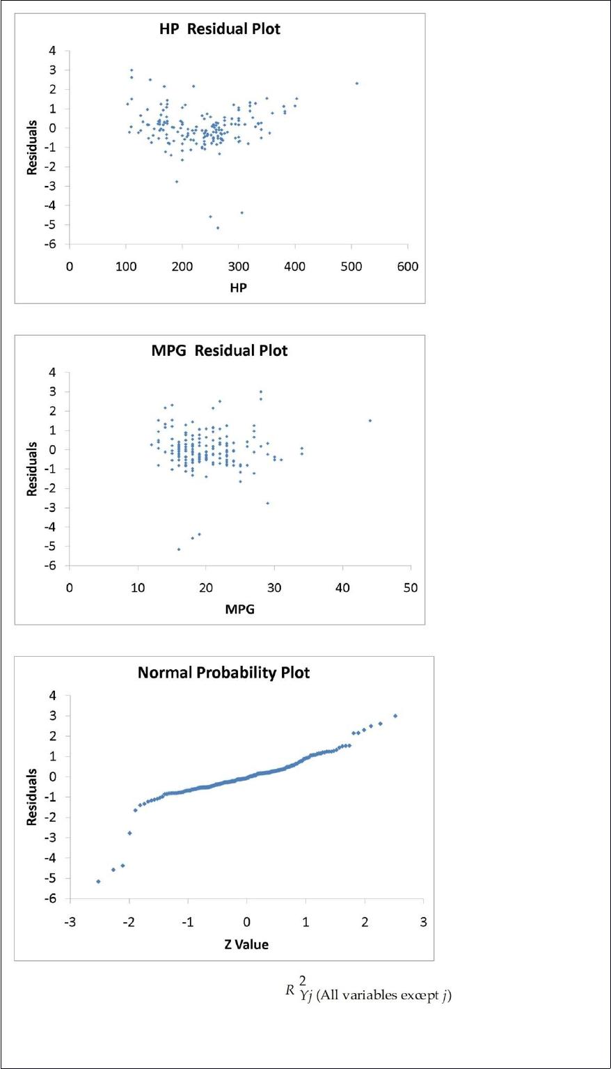
The coefficient of partial determination ( ) of each of the 5
predictors are, respectively, 0.0380, 0.4376, 0.0248, 0.0188, and 0.0312.
The coefficient of multiple determination for the regression model using each of the 5

variables Xj as the dependent variable and all other X variables as independent variables
( ) are, respectively, 0.7461, 0.5676, 0.6764, 0.8582, 0.6632.
Referring to Table 17-9, the 0 to 60 miles per hour acceleration time of a coupe is
predicted to be 0.7679 seconds lower than that of an SUV.
True or False: The test statistic measures how close the computed sample statistic has
come to the hypothesized population parameter.
TABLE 1-1
The manager of the customer service division of a major consumer electronics company
is interested in determining whether the customers who have purchased a Blu-ray
player made by the company over the past 12 months are satisfied with their products.
Referring to Table 1-1, the possible responses to the question “What is your annual
income rounded to the nearest thousands?” are values from a
A) discrete numerical variable.
B) continuous numerical variable.
C) categorical variable.
D) table of random numbers.
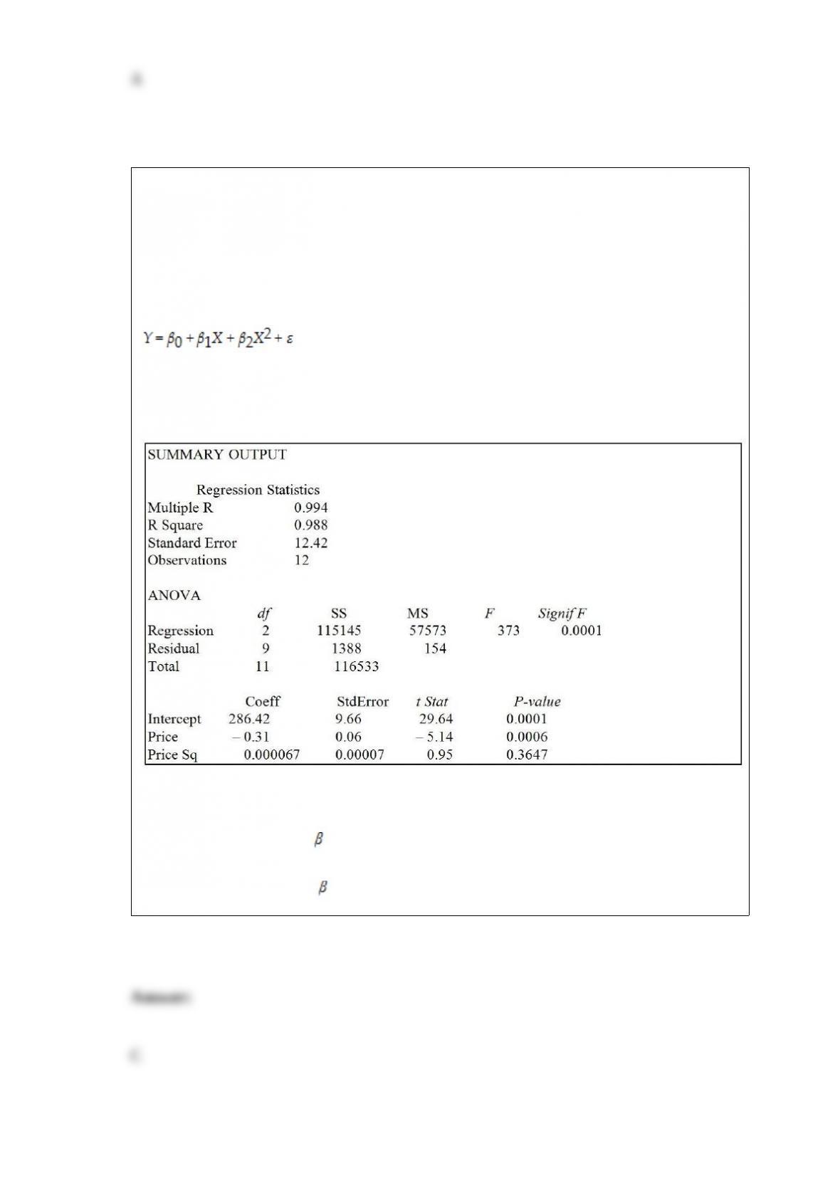
TABLE 15-1
A certain type of rare gem serves as a status symbol for many of its owners. In theory,
for low prices, the demand increases and it decreases as the price of the gem increases.
However, experts hypothesize that when the gem is valued at very high prices, the
demand increases with price due to the status owners believe they gain in obtaining the
gem. Thus, the model proposed to best explain the demand for the gem by its price is
the quadratic model:
where Y = demand (in thousands) and X = retail price per carat.
This model was fit to data collected for a sample of 12 rare gems of this type. A portion
of the computer analysis obtained from Microsoft Excel is shown below:
Referring to Table 15-1, does there appear to be significant upward curvature in the
response curve relating the demand (Y) and the price (X) at 10% level of significance?
A) Yes, since the p-value for the test is less than 0.10.
B) No, since the value of 2 is near 0.
C) No, since the p-value for the test is greater than 0.10.
D) Yes, since the value of 2 is positive.
The logarithm transformation can be used
A) to overcome violations to the autocorrelation assumption.
B) to test for possible violations to the autocorrelation assumption.
C) to overcome violations to the homoscedasticity assumption.
D) to test for possible violations to the homoscedasticity assumption.
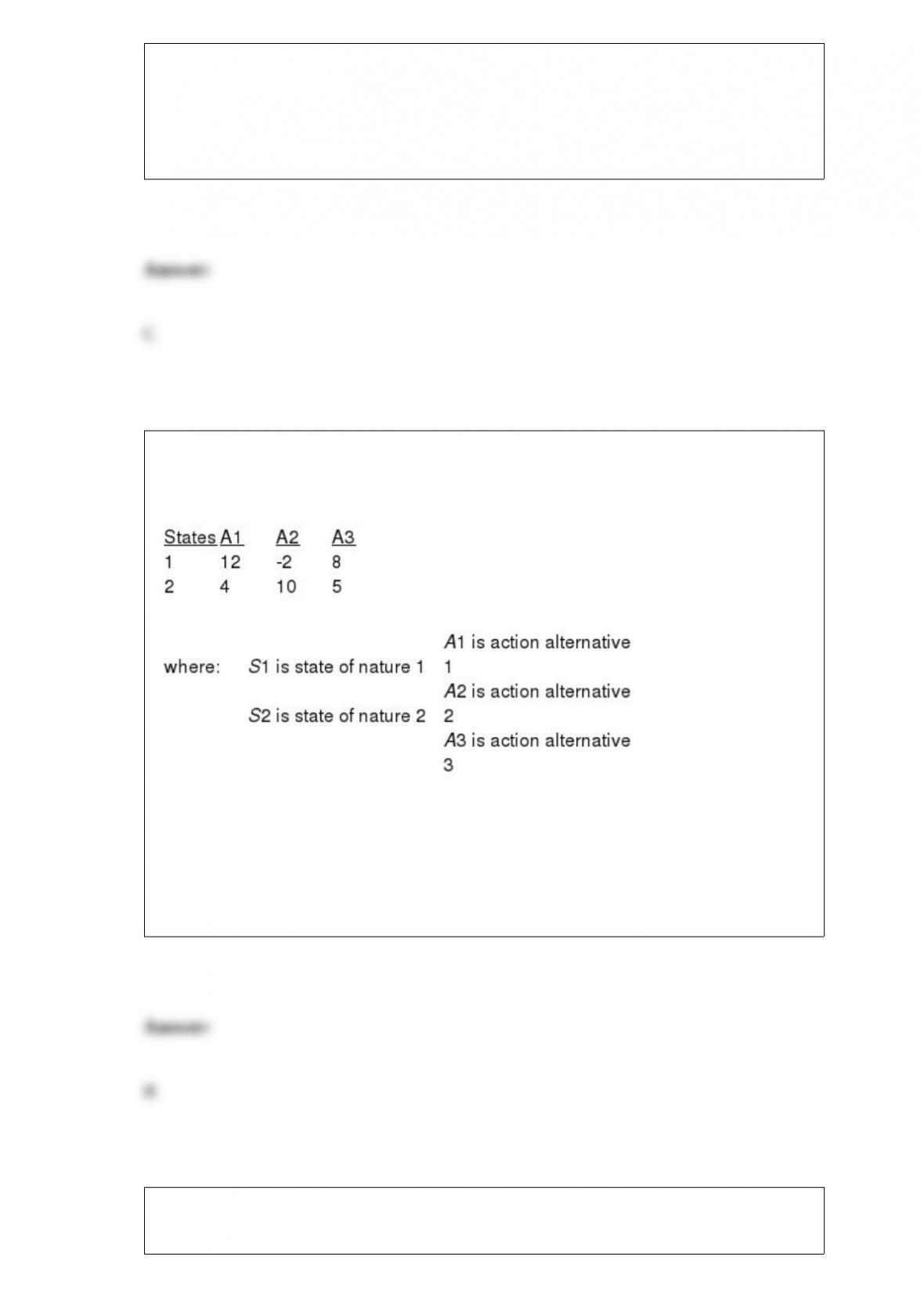
TABLE 19-1
The following payoff table shows profits associated with a set of 3 alternatives under 2
possible states of nature
Referring to Table 19-1, if the probability of S1 is 0.5, then the coefficient of variation
for A1 is
A) 0.231.
B) 0.5.
C) 1.5.
D) 2.
TABLE 10-5
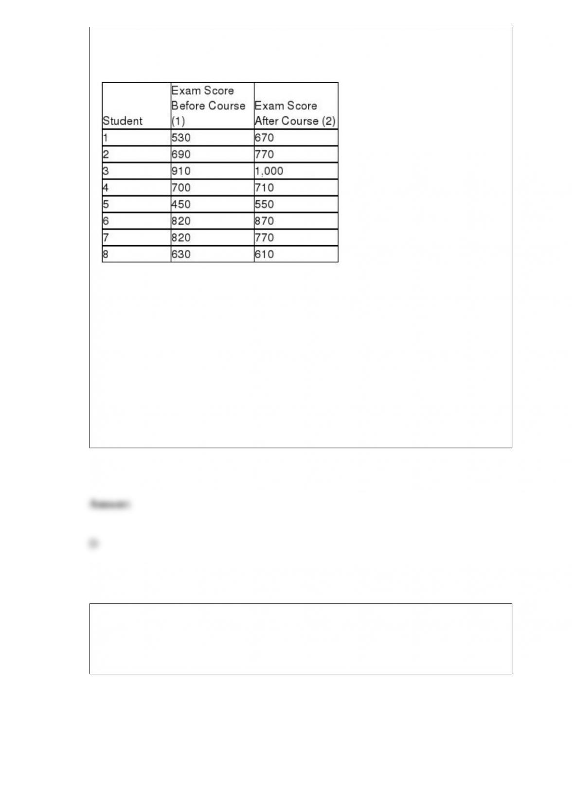
To test the effectiveness of a business school preparation course, 8 students took a
general business test before and after the course. The results are given below.
Referring to Table 10-5, what is the critical value for testing at the 5% level of
significance whether the business school preparation course is effective in improving
exam scores?
A) 2.365
B) 2.145
C) 1.761
D) 1.895
A manufacturer of flashlight batteries took a sample of 130 batteries from a day’s
production and used them continuously until they were drained. The number of hours
until failure were recorded. Given below is the boxplot of the number of hours it took to
drain each of the 130 batteries. The distribution of the number of hours is

A) right-skewed.
B) left-skewed.
C) symmetrical.
D) None of the above.
TABLE 17-2
One of the most common questions of prospective house buyers pertains to the cost of
heating in dollars (Y). To provide its customers with information on that matter, a large
real estate firm used the following 4 variables to predict heating costs: the daily
minimum outside temperature in degrees of Fahrenheit (X1), the amount of insulation in
inches (X2), the number of windows in the house (X3), and the age of the furnace in
years (X4). Given below are the EXCEL outputs of two regression models.
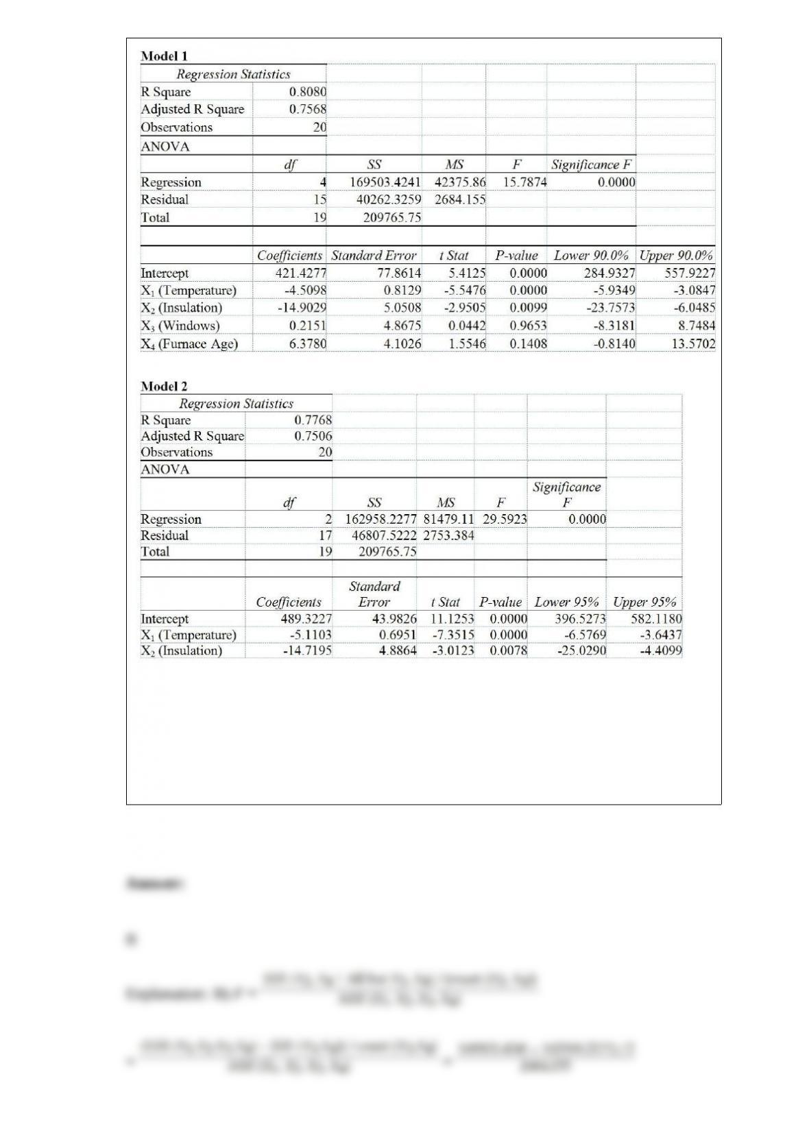
Referring to Table 17-2, what is the value of the partial F test statistic for H0 : β3 = β4 =
0 vs. H1 : At least one βj ≠0, j = 3, 4?
A) 0.820
B) 1.219
C) 1.382
D) 15.787

Data on the amount of money made in a year by 1,000 families in a small town were
collected. You want to know how much each family will get if the money made by all
the 1,000 families is pooled together and then evenly redistributed back to them. Which
of the following would you compute?
A) Arithmetic mean
B) Median
C) Interquartile range
D) Coefficient of correlation
TABLE 17-6
A weight-loss clinic wants to use regression analysis to build a model for weight loss of
a client (measured in pounds). Two variables thought to affect weight loss are client’s
length of time on the weight-loss program and time of session. These variables are
described below:
Y = Weight loss (in pounds)
X1 = Length of time in weight-loss program (in months)
X2 = 1 if morning session, 0 if not
X3 = 1 if afternoon session, 0 if not (Base level = evening session)
Data for 12 clients on a weight-loss program at the clinic were collected and used to fit
the interaction model:
Y = β0 + β1X1 + β2X2 + β3X3 + β4X1X2 + β5X1X3 + ε
Partial output from Microsoft Excel follows:
Regression Statistics
ANOVA
F = 5.41118 Significance F = 0.040201
Referring to Table 17-6, in terms of the βs in the model, give the mean change in
weight loss (Y) for every 1-month increase in time in the program (X1) when attending
the evening session.
A) β1+ β4
B) β1 + β5
C) β1
D) β4 + β5
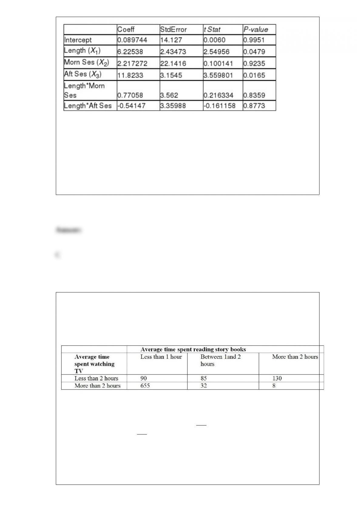
TABLE 12-12
Parents complain that children read too few storybooks and watch too much television
nowadays. A survey of 1,000 children reveals the following information on average
time spent watching TV and average time spent reading storybooks.
Referring to Table 12-12, we want to test whether there is any relationship between
average time spent watching TV and average time spent reading storybooks. Suppose
the value of the test statistic was 164 (which is not the correct answer) and the critical
value was 19.00 (which is not the correct answer), then we could conclude that
A) there is a connection between time spent reading storybooks and time spent
watching TV.
B) there is no connection between time spent reading storybooks and time spent

watching TV.
C) more time spent reading storybooks leads to less time spent watching TV.
D) more time spent watching TV leads to less time spent reading storybooks.
Suppose a 95% confidence interval for turns out to be (1,000, 2,100). Give a
definition of what it means to be “95% confident” as an inference.
A) In repeated sampling, the population parameter would fall in the given interval 95%
of the time.
B) In repeated sampling, 95% of the intervals constructed would contain the population
mean.
C) 95% of the observations in the entire population fall in the given interval.
D) 95% of the observations in the sample fall in the given interval.
Referring to Table 14-4, which of the following values for the level of significance is
the smallest for which each explanatory variable is significant individually?
TABLE 14-4
A real estate builder wishes to determine how house size (House) is influenced by
family income (Income) and family size (Size). House size is measured in hundreds of
square feet and income is measured in thousands of dollars. The builder randomly
selected 50 families and ran the multiple regression. Partial Microsoft Excel output is
provided below:
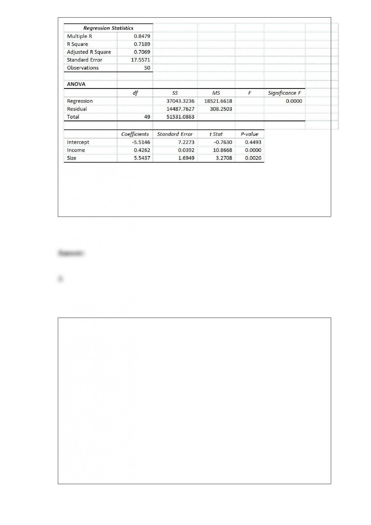
Also SSR (X1∣ X2) = 36400.6326 and SSR (X2∣ X1) = 3297.7917
A) 0.001
B) 0.010
C) 0.025
D) 0.050
TABLE 11-8
A physician and president of a Tampa Health Maintenance Organization (HMO) are
attempting to show the benefits of managed health care to an insurance company. The
physician believes that certain types of doctors are more cost-effective than others. One
theory is that Primary Specialty is an important factor in measuring the
cost-effectiveness of physicians. To investigate this, the president obtained independent
random samples of 20 HMO physicians from each of 4 primary specialties – General
Practice (GP), Internal Medicine (IM), Pediatrics (PED), and Family Physicians (FP) –
and recorded the total charges per member per month for each. A second factor which
the president believes influences total charges per member per month is whether the
doctor is a foreign or USA medical school graduate. The president theorizes that foreign
graduates will have higher mean charges than USA graduates. To investigate this, the
president also collected data on 20 foreign medical school graduates in each of the 4
primary specialty types described above. So information on charges for 40 doctors (20
foreign and 20 USA medical school graduates) was obtained for each of the 4
specialties. The results for the ANOVA are summarized in the following table.
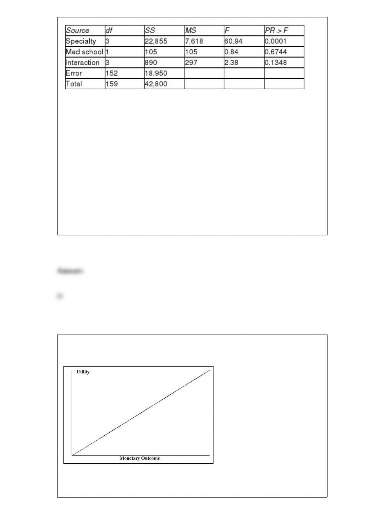
Referring to Table 11-8, what assumption(s) need(s) to be made in order to conduct the
test for differences between the mean charges of foreign and USA medical school
graduates?
A) There is no significant interaction effect between the area of primary specialty and
the medical school on the doctors’ mean charges.
B) The charges in each group of doctors sampled are drawn from normally distributed
populations.
C) The charges in each group of doctors sampled are drawn from populations with
equal variances.
D) All of the above are necessary assumptions.
Look at the utility function graphed below and select the type of decision maker that
corresponds to the graph.
A) Risk averter
B) Risk neutral
C) Risk taker
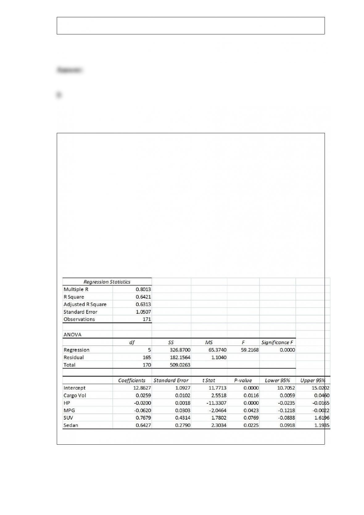
D) Risk player
TABLE 17-9
What are the factors that determine the acceleration time (in sec.) from 0 to 60 miles per
hour of a car? Data on the following variables for 171 different vehicle models were
collected:
Accel Time: Acceleration time in sec.
Cargo Vol: Cargo volume in cu. ft.
HP: Horsepower
MPG: Miles per gallon
SUV: 1 if the vehicle model is an SUV with Coupe as the base when SUV and Sedan
are both 0
Sedan: 1 if the vehicle model is a sedan with Coupe as the base when SUV and Sedan
are both 0
The regression results using acceleration time as the dependent variable and the
remaining variables as the independent variables are presented below.
The various residual plots are as shown below.
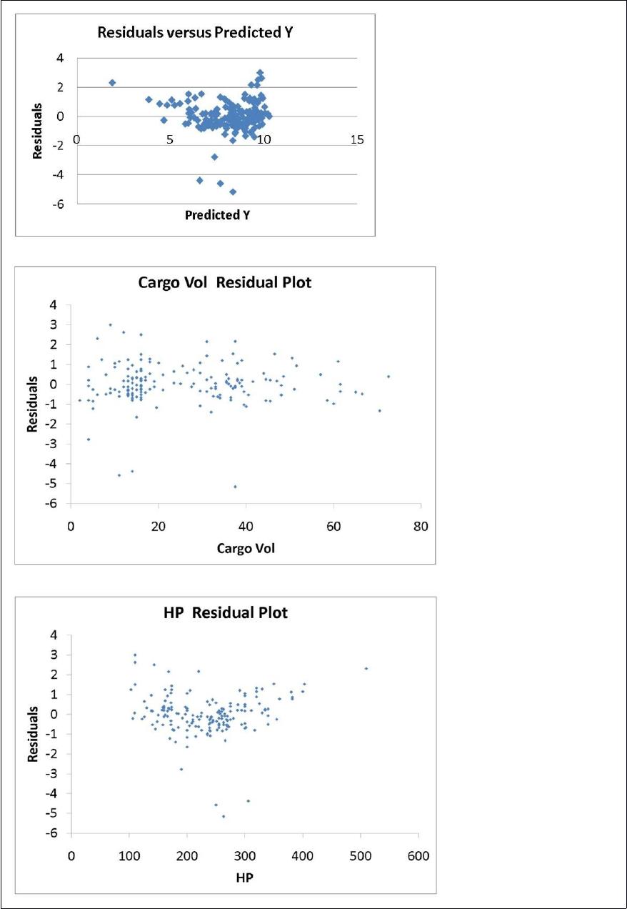
The coefficient of partial determination ( ) of each of the 5
predictors are, respectively, 0.0380, 0.4376, 0.0248, 0.0188, and 0.0312.
The coefficient of multiple determination for the regression model using each of the 5
variables Xj as the dependent variable and all other X variables as independent variables
( ) are, respectively, 0.7461, 0.5676, 0.6764, 0.8582, 0.6632.
Referring to Table 17-9, what is the correct interpretation for the estimated coefficient
for Sedan?
A) The mean 0 to 60 miles per hour acceleration time of a sedan is estimated to be
0.6427 seconds higher than that of a coupe after considering the effect of all the other
independent variables in the model.
B) The mean 0 to 60 miles per hour acceleration time of a sedan is estimated to be
0.6427 seconds higher than that of an SUV after considering the effect of all the other
independent variables in the model.
C) The mean 0 to 60 miles per hour acceleration time of a sedan is estimated to be
0.6427 seconds lower than that of a coupe after considering the effect of all the other
independent variables in the model.
D) The mean 0 to 60 miles per hour acceleration time of a sedan is estimated to be
0.6427 seconds lower than that of an SUV after considering the effect of all the other
independent variables in the model.
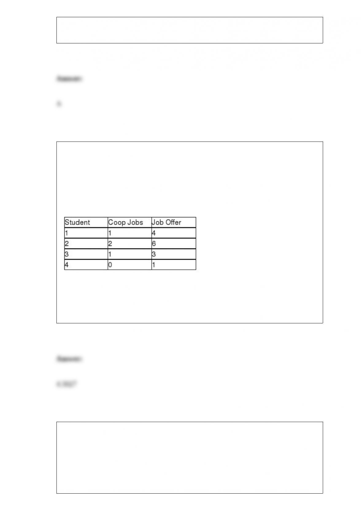
TABLE 13-3
The director of cooperative education at a state college wants to examine the effect of
cooperative education job experience on marketability in the work place. She takes a
random sample of 4 students. For these 4, she finds out how many times each had a
cooperative education job and how many job offers they received upon graduation.
These data are presented in the table below.
Referring to Table 13-3, suppose the director of cooperative education wants to
construct a 95% confidence-interval estimate for the mean number of job offers
received by students who have had exactly one cooperative education job. The t critical
value she would use is ________.
TABLE 17-10
Given below are results from the regression analysis where the dependent variable is
the number of weeks a worker is unemployed due to a layoff (Unemploy) and the
independent variables are the age of the worker (Age), the number of years of education
received (Edu), the number of years at the previous job (Job Yr), a dummy variable for
marital status (Married: 1 = married, 0 = otherwise), a dummy variable for head of
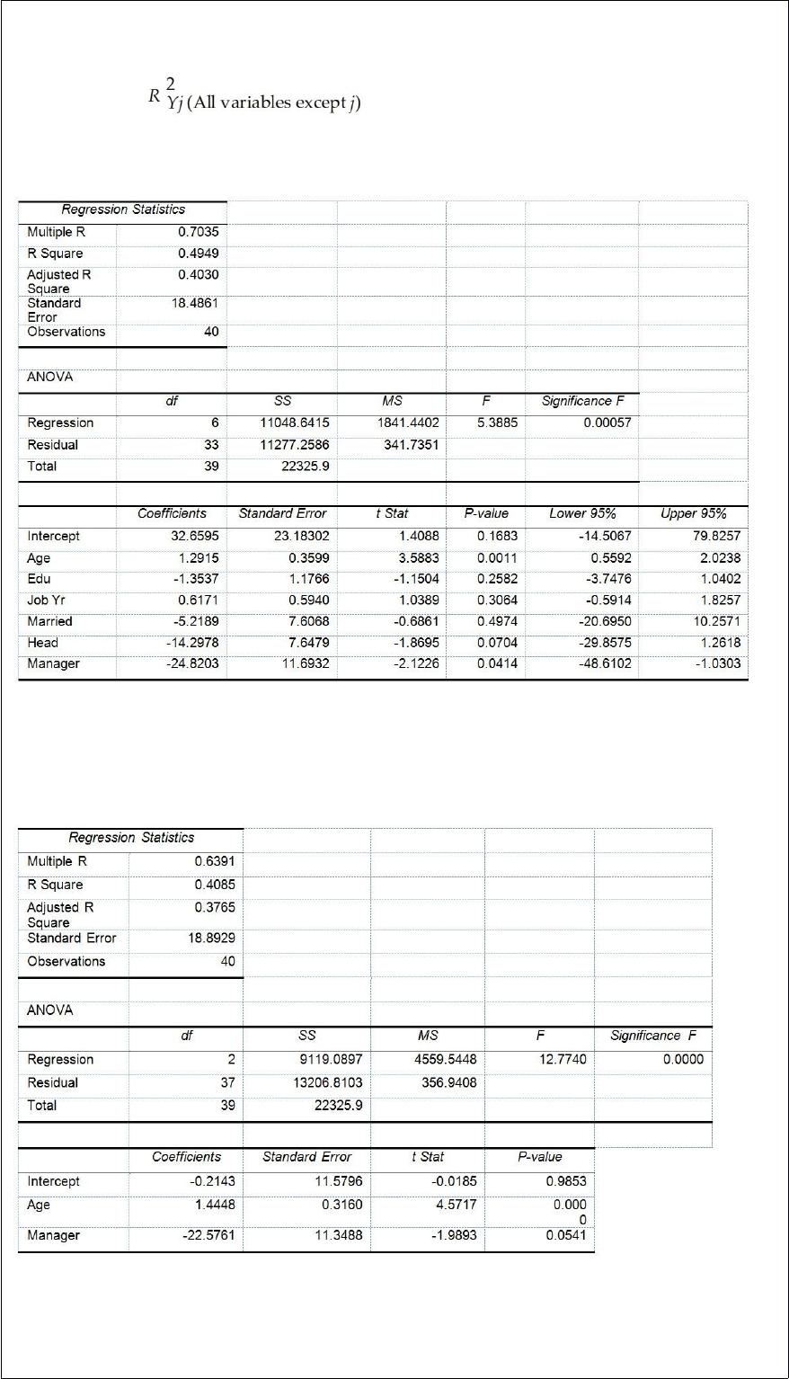
household (Head: 1 = yes, 0 = no) and a dummy variable for management position
(Manager: 1 = yes, 0 = no). We shall call this Model 1. The coefficient of partial
determination ( ) of each of the 6 predictors are, respectively,
0.2807, 0.0386, 0.0317, 0.0141, 0.0958, and 0.1201.
Model 2 is the regression analysis where the dependent variable is Unemploy and the
independent variables are Age and Manager. The results of the regression analysis are
given below:
Referring to Table 17-10, Model 1, what is the value of the test statistic when testing
whether age has any effect on the number of weeks a worker is unemployed due to a
layoff while holding constant the effect of all the other independent variables?

TABLE 9-10
A manufacturer produces light bulbs that have a mean life of at least 500 hours when
the production process is working properly. Based on past experience, the population
standard deviation is 50 hours and the light bulb life is normally distributed. The
operations manager stops the production process if there is evidence that the population
mean light bulb life is below 500 hours.
Referring to Table 9-10, if you select a sample of 100 light bulbs and are willing to have
a level of significance of 0.10, the power of the test is ________ if the population mean
bulb life is 490 hours.
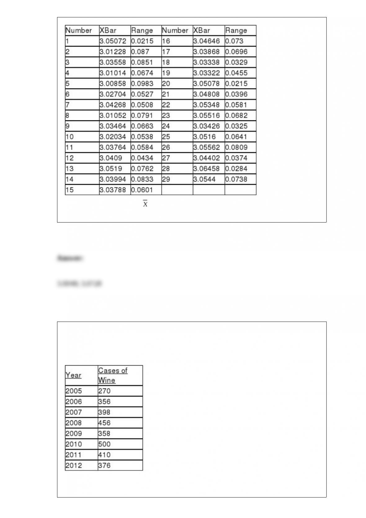
TABLE 18-9
The manufacturer of canned food constructed control charts and analyzed several
quality characteristics. One characteristic of interest is the weight of the filled cans. The
lower specification limit for weight is 2.95 pounds. The table below provides the range
and mean of the weights of five cans tested every fifteen minutes during a day’s
production.
Referring to Table 18-9, an chart is to be used for the weight. The lower control limit
for this data set is ________, while the upper control limit is ________.
TABLE 16-4
The number of cases of merlot wine sold by a Paso Robles winery in an 8-year period
follows.
Referring to Table 16-4, a centered 5-year moving average is to be constructed for the
wine sales. The moving average for 2007 is ________.
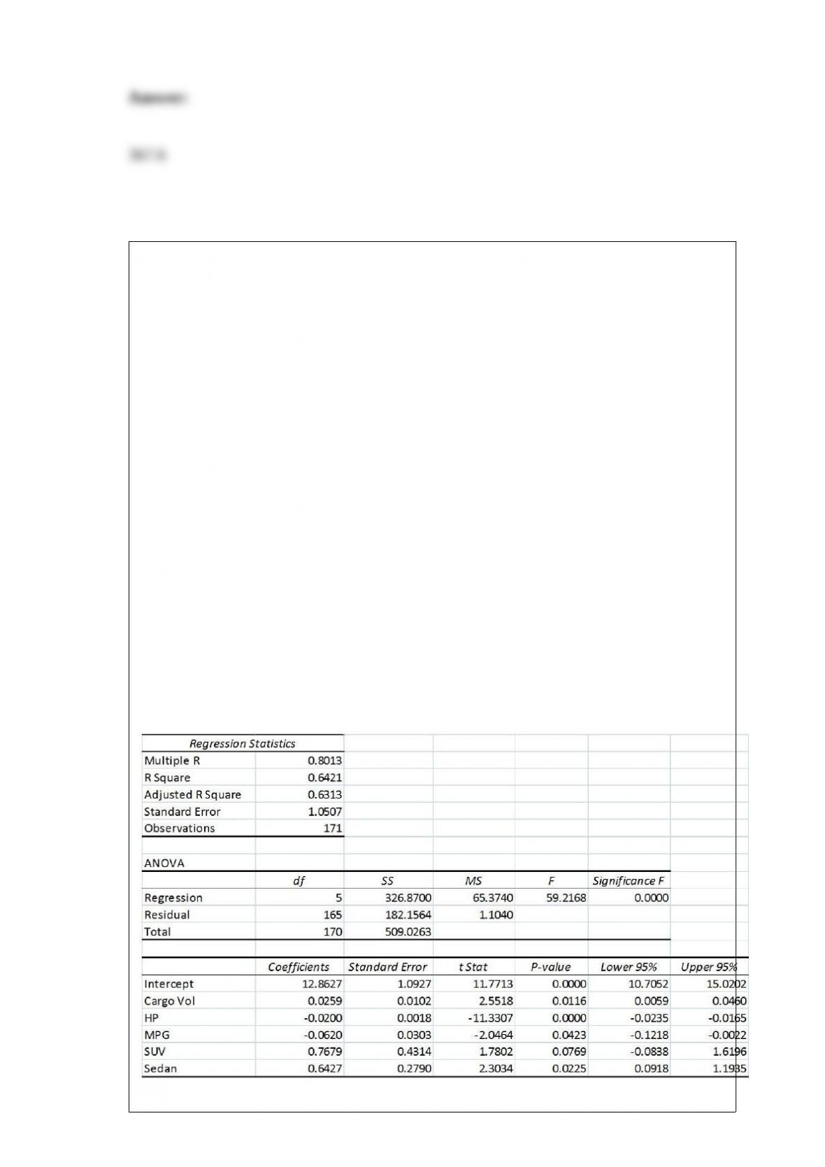
TABLE 17-9
What are the factors that determine the acceleration time (in sec.) from 0 to 60 miles per
hour of a car? Data on the following variables for 171 different vehicle models were
collected:
Accel Time: Acceleration time in sec.
Cargo Vol: Cargo volume in cu. ft.
HP: Horsepower
MPG: Miles per gallon
SUV: 1 if the vehicle model is an SUV with Coupe as the base when SUV and Sedan
are both 0
Sedan: 1 if the vehicle model is a sedan with Coupe as the base when SUV and Sedan
are both 0
The regression results using acceleration time as the dependent variable and the
remaining variables as the independent variables are presented below.
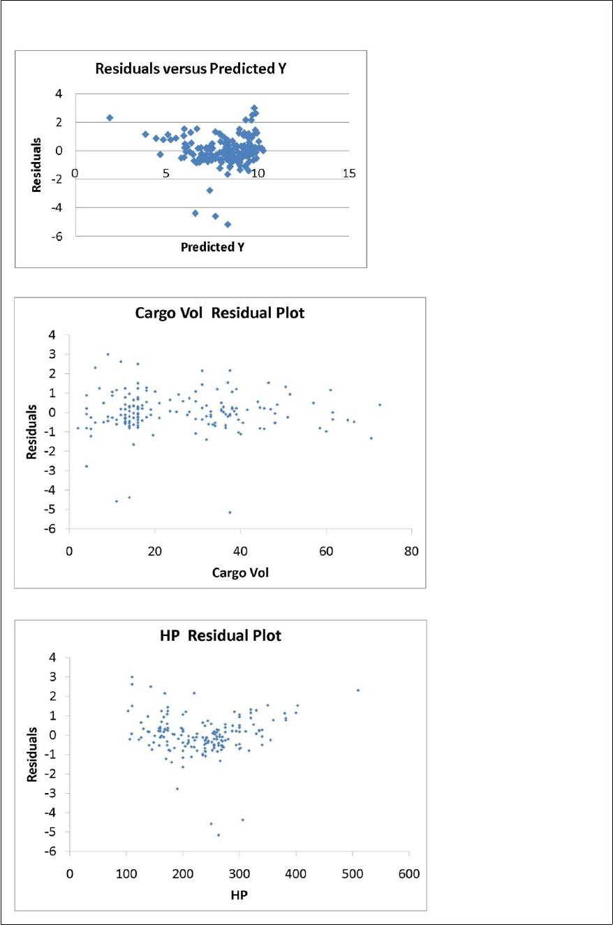
The various residual plots are as shown below.
The coefficient of partial determination ( ) of each of the 5
predictors are, respectively, 0.0380, 0.4376, 0.0248, 0.0188, and 0.0312.
The coefficient of multiple determination for the regression model using each of the 5
variables Xj as the dependent variable and all other X variables as independent variables
( ) are, respectively, 0.7461, 0.5676, 0.6764, 0.8582, 0.6632.
Referring to Table 17-9, what is the p-value of the test statistic to determine whether HP
makes a significant contribution to the regression model in the presence of the other
independent variables at a 5% level of significance?

TABLE 8-4
The actual voltages of power packs labeled as 12 volts are as follows: 11.77, 11.90,
11.64, 11.84, 12.13, 11.99, and 11.77.
Referring to Table 8-4, a confidence interval for this sample would be based on the t
distribution with ________ degrees of freedom.