
TABLE 14-18
A logistic regression model was estimated in order to predict the
probability that a randomly chosen university or college would be a
private university using information on mean total Scholastic Aptitude
Test score (SAT) at the university or college and whether the TOEFL
criterion is at least 90 (Toe90 = 1 if yes, 0 otherwise). The
dependent variable, Y, is school type (Type = 1 if private and 0
otherwise).
The PHStat output is given below:
True or False: Referring to Table 14-18, the null hypothesis that the
model is a good-.tting model cannot be rejected when allowing for a
5% probability of making a type I error.
True or False: In a two-factor ANOVA analysis, the sum of squares due to both factors,
the interaction sum of squares and the within sum of squares must add up to the total
sum of squares.
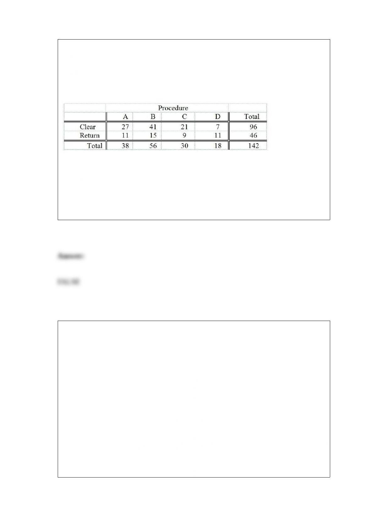
TABLE 12-5
Four surgical procedures currently are used to install pacemakers. If the patient does not
need to return for follow-up surgery, the operation is called a “clear” operation. A heart
center wants to compare the proportion of clear operations for the 4 procedures, and
collects the following numbers of patients from their own records:
They will use this information to test for a difference among the proportion of clear
operations using a chi-square test with a level of significance of 0.05.
True or False: Referring to Table 12-5, there is sufficient evidence to conclude that the
proportions between procedure C and procedure D are different at a 0.05 level of
significance.
TABLE 9-7
A major home improvement store conducted its biggest brand recognition campaign in
the company’s history. A series of new television advertisements featuring well-known
entertainers and sports figures were launched. A key metric for the success of television
advertisements is the proportion of viewers who “like the ads a lot”. A study of 1,189
adults who viewed the ads reported that 230 indicated that they “like the ads a lot.” The
percentage of a typical television advertisement receiving the “like the ads a lot” score
is believed to be 22%. Company officials wanted to know if there is evidence that the
series of television advertisements are less successful than the typical ad (i.e. if there is
evidence that the population proportion of “like the ads a lot” for the company’s ads is
less than 0.22) at a 0.01 level of significance.
True or False: Referring to Table 9-7, the company officials can conclude that there is
sufficient evidence to show that the series of television advertisements are less
successful than the typical ad using a level of significance of 0.01.

True or False: One of the consequences of collinearity in multiple regression is biased
estimates on the slope coefficients.
TABLE 12-2
The dean of a college is interested in the proportion of graduates from his college who
have a job offer on graduation day. He is particularly interested in seeing if there is a
difference in this proportion for accounting and economics majors. In a random sample
of 100 of each type of major at graduation, he found that 65 accounting majors and 52
economics majors had job offers. If the accounting majors are designated as “Group 1”
and the economics majors are designated as “Group 2,” perform the appropriate
hypothesis test using a level of significance of 0.05.
True or False: Referring to Table 12-2, the same decision would be made with this test
if the level of significance had been 0.01 rather than 0.05.
TABLE 14-18
A logistic regression model was estimated in order to predict the
probability that a randomly chosen university or college would be a
private university using information on mean total Scholastic Aptitude
Test score (SAT) at the university or college and whether the TOEFL

criterion is at least 90 (Toe90 = 1 if yes, 0 otherwise). The
dependent variable, Y, is school type (Type = 1 if private and 0
otherwise).
The PHStat output is given below:
True or False: Referring to Table 14-18, there is not enough evidence
to conclude that the model is not a good-.tting model at a 0.05 level
of signi.cance.
A Paso Robles wine producer wanted to forecast the cases of Merlot wine sold. The
number of cases of merlot wine sold in a 28-year period was collected. Which of the
following would be the most appropriate analysis to perform?
A) The Marascuilo Procedure
B) The Tukey-Kramer Procedure
C) Least-squares forecasting with monthly or quarterly data
D) Exponential smoothing modeling
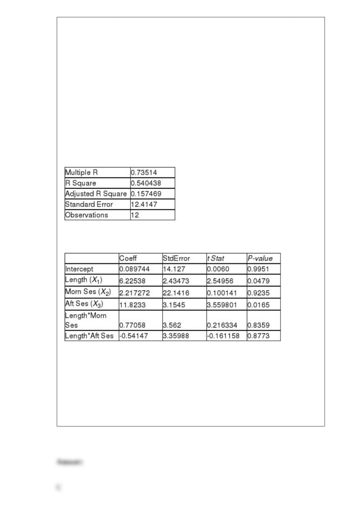
TABLE 17-6
A weight-loss clinic wants to use regression analysis to build a model for weight loss of
a client (measured in pounds). Two variables thought to affect weight loss are client’s
length of time on the weight-loss program and time of session. These variables are
described below:
Y = Weight loss (in pounds)
X1 = Length of time in weight-loss program (in months)
X2 = 1 if morning session, 0 if not
X3 = 1 if afternoon session, 0 if not (Base level = evening session)
Data for 12 clients on a weight-loss program at the clinic were collected and used to fit
the interaction model:
Y = β0 + β1X1 + β2X2 + β3X3 + β4X1X2 + β5X1X3 + ε
Partial output from Microsoft Excel follows:
Regression Statistics
ANOVA
F = 5.41118 Significance F = 0.040201
Referring to Table 17-6, in terms of the βs in the model, give the mean change in
weight loss (Y) for every 1-month increase in time in the program (X1) when attending
the evening session.
A) β1+ β4
B) β1 + β5
C) β1
D) β4 + β5
If a particular set of data is approximately normally distributed, we would find that
approximately
A) 2 of every 3 observations would fall between 1 standard deviation around the
mean.
B) 4 of every 5 observations would fall between 1.28 standard deviations around the
mean.
C) 19 of every 20 observations would fall between 2 standard deviations around the
mean.
D) All of the above.
If two equally likely events A and B are mutually exclusive and collectively exhaustive,
what is the probability that event A occurs?
A) 0
B) 0.50
C) 1.00
D) Cannot be determined from the information given.
TABLE 12-14
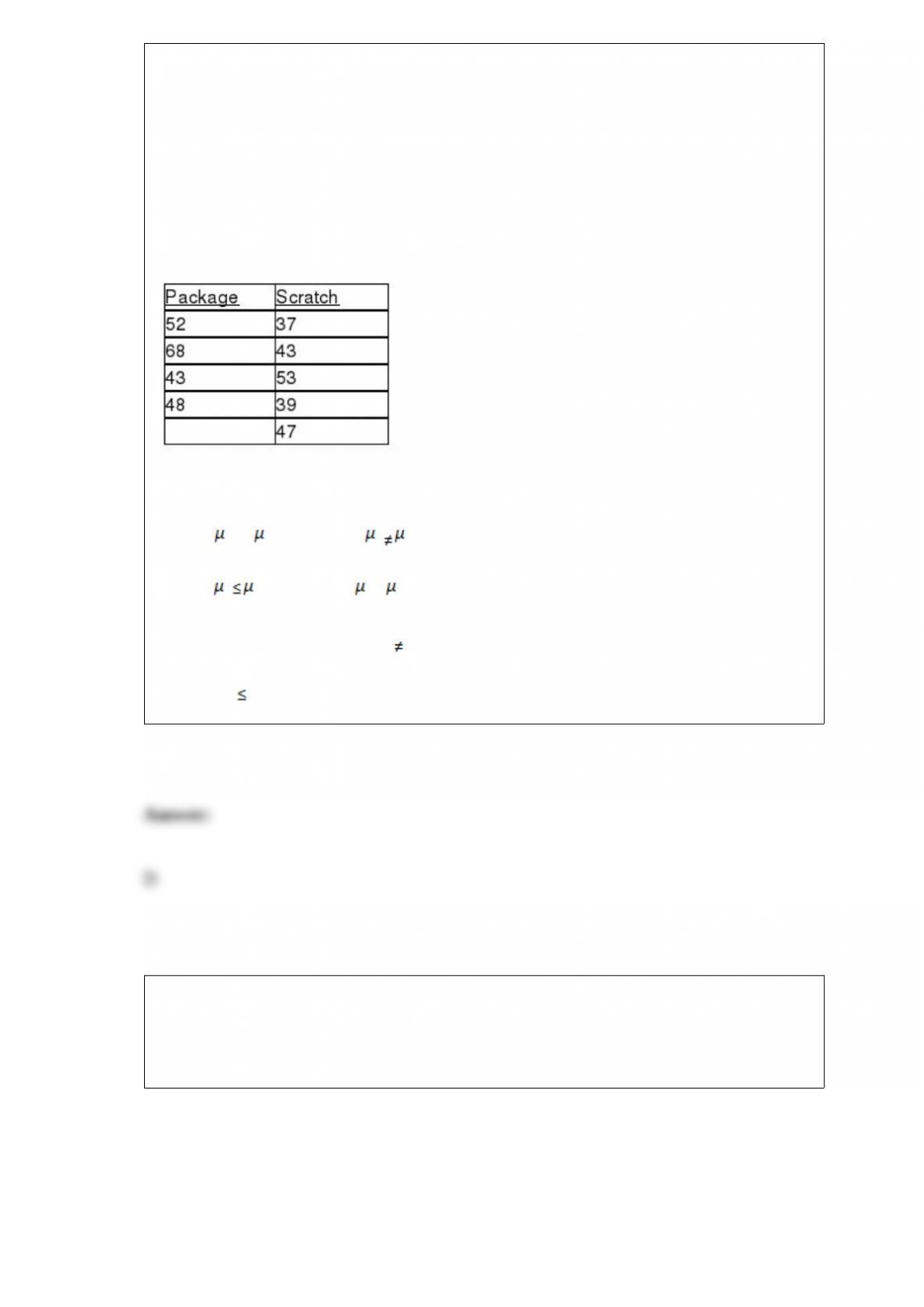
A perfume manufacturer is trying to choose between 2 magazine advertising layouts.
An expensive layout would include a small package of the perfume. A cheaper layout
would include a ‘scratch-and-sniff” sample of the product. The manufacturer would use
the more expensive layout only if there is evidence that it would lead to a higher
approval rate. The manufacturer presents the more expensive layout to 4 groups and
determines the approval rating for each group. He presents the ‘scratch-and-sniff” layout
to 5 groups and again determines the approval rating of the perfume for each group. The
data are given below. Use this to test the appropriate hypotheses with the Wilcoxon
Rank Sum Test with a level of significance of 0.05.
Referring to Table 12-14, the hypotheses that should be used are
A) H0 : 1 = 2 versus H1 : 1 2.
B) H0 : 1 2 versus H1 : 1 > 2.
C) H0 : M1 = M2 versus H1 : M1M2.
D) H0 : M1M2 versus H1 : M1 >M2.
TABLE 2-5
The following are the duration in minutes of a sample of long-distance phone calls
made within the continental United States reported by one long-distance carrier.
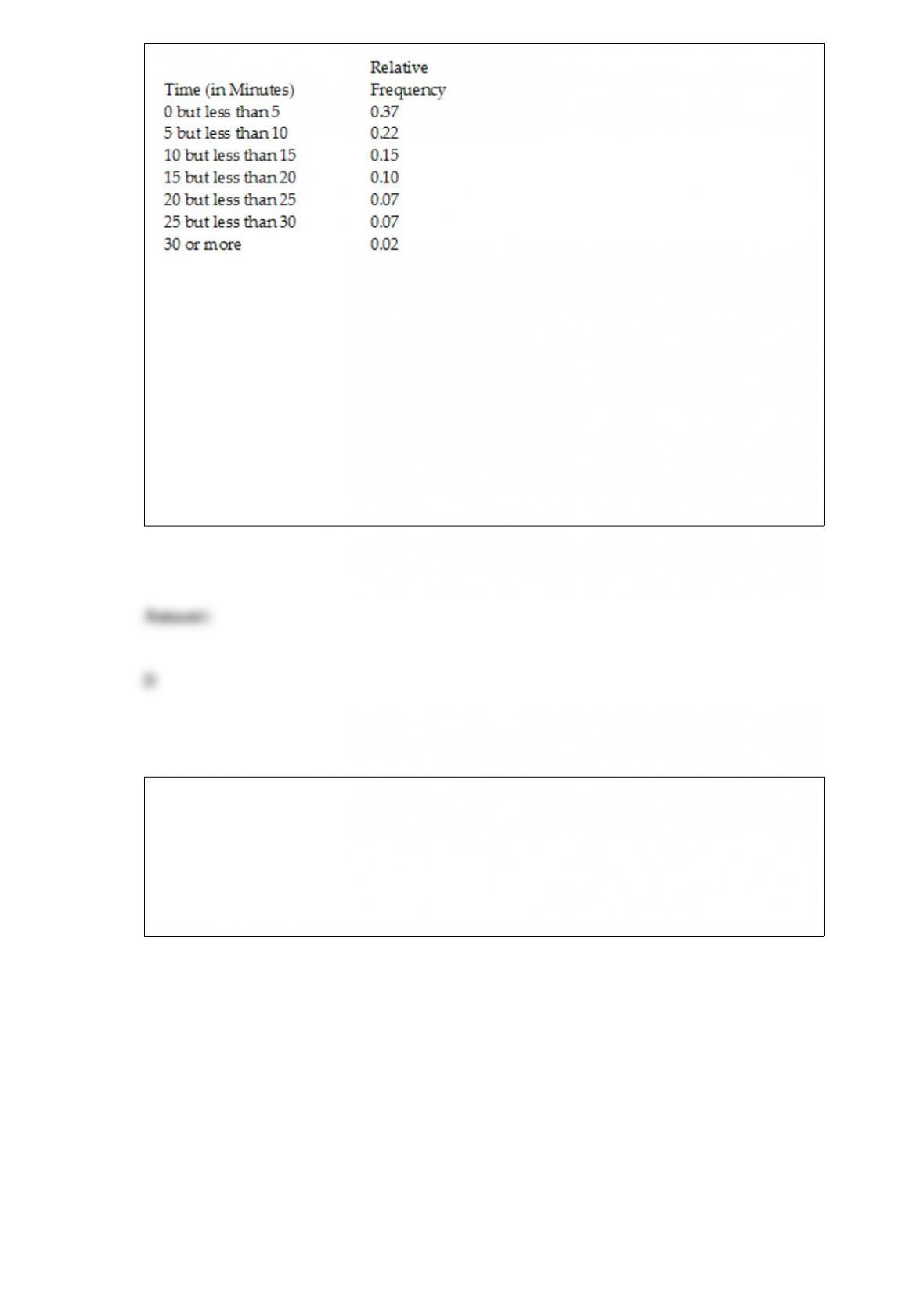
Referring to Table 2-5, if 10 calls lasted 30 minutes or more, how many calls lasted less
than 5 minutes?
A) 10
B) 185
C) 295
D) 500
TABLE 17-1
A real estate builder wishes to determine how house size (House) is influenced by
family income (Income), family size (Size), and education of the head of household
(School). House size is measured in hundreds of square feet, income is measured in
thousands of dollars, and education is in years. The builder randomly selected 50
families and ran the multiple regression. Microsoft Excel output is provided below:
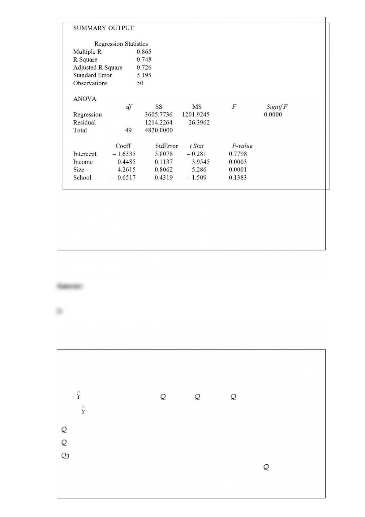
Referring to Table 17-1, which of the following values for the level of significance is
the smallest for which every explanatory variable is significant individually?
A) 0.01
B) 0.025
C) 0.05
D) 0.15
TABLE 16-12
A local store developed a multiplicative time-series model to forecast its revenues in
future quarters, using quarterly data on its revenues during the 5-year period from 2008
to 2012. The following is the resulting regression equation:
log10 = 6.102 + 0.012 X – 0.129 1 – 0.054 2 + 0.098 3
where is the estimated number of contracts in a quarter
X is the coded quarterly value with X = 0 in the first quarter of 2008
1 is a dummy variable equal to 1 in the first quarter of a year and 0 otherwise
2 is a dummy variable equal to 1 in the second quarter of a year and 0 otherwise
is a dummy variable equal to 1 in the third quarter of a year and 0 otherwise
Referring to Table 16-12, the best interpretation of the coefficient of 2 (-0.054) in the
regression equation is
A) the revenues in the second quarter of a year is approximately 5.4% lower than the
average over all 4 quarters.
B) the revenues in the second quarter of a year is approximately 5.4% lower than it
would be during the fourth quarter.
C) the revenues in the second quarter of a year is approximately 11.69% lower than the
average over all 4 quarters.
D) the revenues in the second quarter of a year is approximately 11.69% lower than it
would be during the fourth quarter.
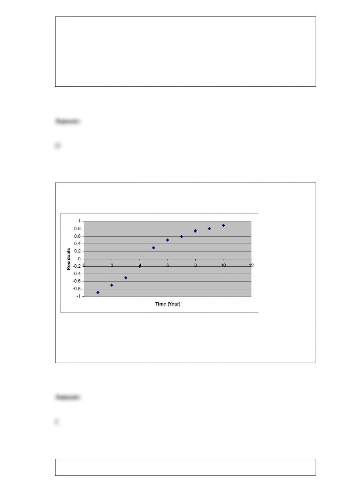
After estimating a trend model for annual time-series data, you obtain the following
residual plot against time.
The problem with your model is that
A) the cyclical component has not been accounted for.
B) the seasonal component has not been accounted for.
C) the trend component has not been accounted for.
D) the irregular component has not been accounted for.
To demonstrate a sampling method, the instructor in a class picked the first 5 students
sitting in the last row of the class. This is an example of a
A) systematic sample.
B) simple random sample.
C) stratified sample.
D) convenience sample.
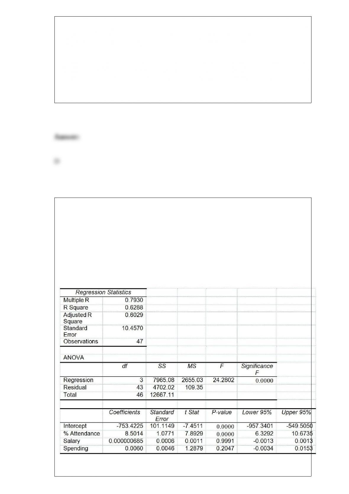
TABLE 17-8
The superintendent of a school district wanted to predict the percentage of students
passing a sixth-grade proficiency test. She obtained the data on percentage of students
passing the proficiency test (% Passing), daily mean of the percentage of students
attending class (% Attendance), mean teacher salary in dollars (Salaries), and
instructional spending per pupil in dollars (Spending) of 47 schools in the state.
Following is the multiple regression output with Y = % Passing as the dependent
variable, X1 = % Attendance, X2 = Salaries and X3 = Spending:
Referring to Table 17-8, which of the following is a correct statement?
A) 62.88% of the total variation in the percentage of students passing the proficiency

test can be explained by daily mean of the percentage of students attending class, mean
teacher salary, and instructional spending per pupil.
B) 62.88% of the total variation in the percentage of students passing the proficiency
test can be explained by daily mean of the percentage of students attending class, mean
teacher salary, and instructional spending per pupil after adjusting for the number of
predictors and sample size.
C) 62.88% of the total variation in the percentage of students passing the proficiency
test can be explained by daily mean of the percentage of students attending class
holding constant the effect of mean teacher salary, and instructional spending per pupil.
D) 62.88% of the total variation in the percentage of students passing the proficiency
test can be explained by daily mean of the percentage of students attending class after
adjusting for the effect of mean teacher salary, and instructional spending per pupil.
The oranges grown in corporate farms in an agricultural state were damaged by some
unknown fungi a few years ago. Suppose the manager of a large farm wanted to study
the impact of the fungi on the orange crops on a daily basis over a 6-week period. On
each day a random sample of orange trees was selected from within a random sample of
acres. The daily average number of damaged oranges per tree and the proportion of
trees having damaged oranges were calculated. The two main measures calculated each
day (i.e., average number of damaged oranges per tree and proportion of trees having
damaged oranges) may be used on a daily basis to estimate the respective true
population ________.
TABLE 14-10
You worked as an intern at We Always Win Car Insurance Company
last summer. You notice that individual car insurance premiums
depend very much on the age of the individual and the number of
traffic tickets received by the individual. You performed a regression
analysis in EXCEL and obtained the following partial information:

Referring to Table 14-10, the proportion of the total variability in
insurance premiums that can be explained by AGE and TICKETS after
adjusting for the number of observations and the number
independent variables is ________.
An insurance company evaluates many numerical variables about a person before
deciding on an appropriate rate for automobile insurance. The number of tickets a
person has received in the last 3 years is an example of a ________ numerical variable.
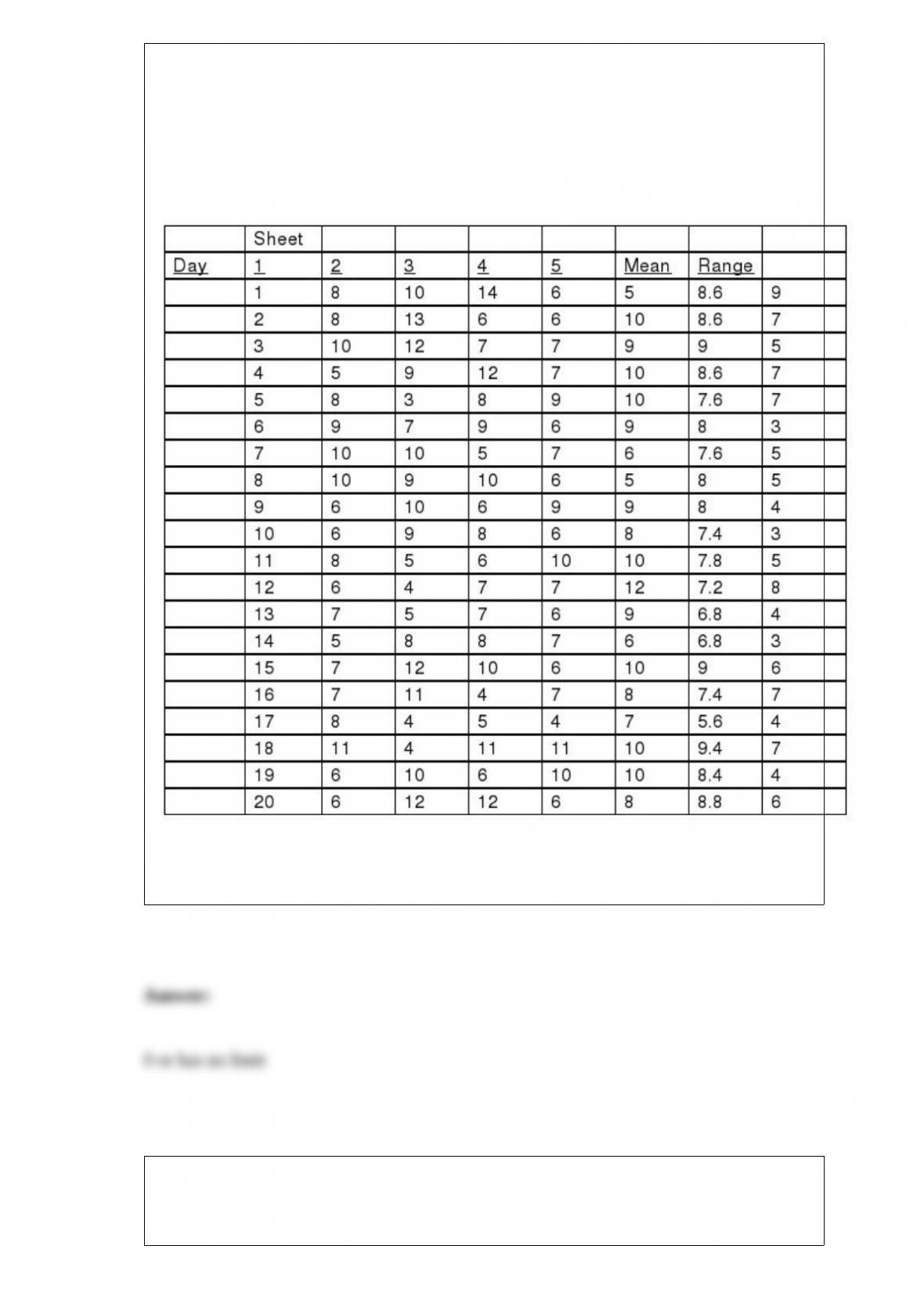
TABLE 18-7
A supplier of silicone sheets for producers of computer chips wants to evaluate her
manufacturing process. She takes sample sizes of 5 from each day’s output and counts
the number of blemishes on each silicone sheet. The results from 20 days of such
evaluations are presented below.
She also decides that the upper specification limit is 10 blemishes.
Referring to Table 18-7, an R chart is to be constructed for the number of blemishes.
The lower control limit for this data set is ________.
TABLE 5-7
There are two houses with almost identical characteristics available for investment in
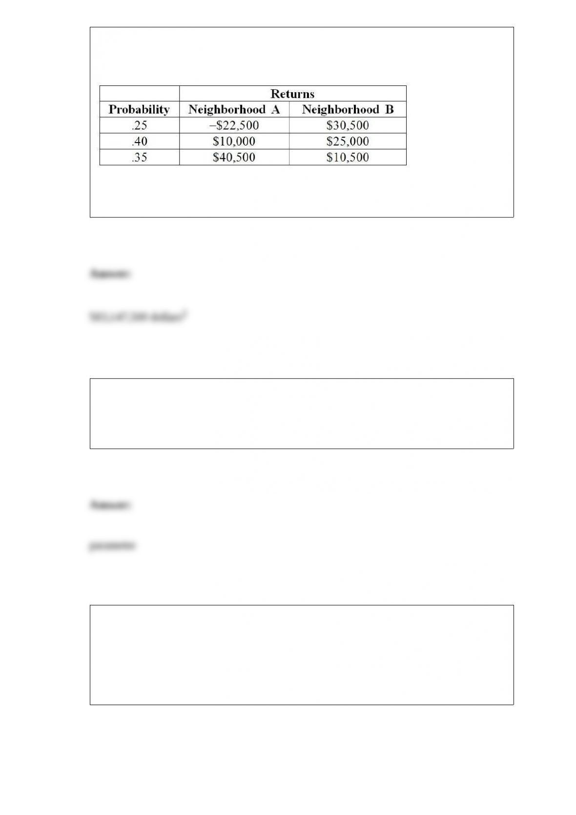
two different neighborhoods with drastically different demographic composition. The
anticipated gain in value when the houses are sold in 10 years has the following
probability distribution:
Referring to Table 5-7, what is the variance of the gain in value for the house in
neighborhood A?
The Commissioner of Health in New York State wanted to study malpractice litigation
in New York. A sample of 31 thousand medical records was drawn from a population of
2.7 million patients who were discharged during 2010. The true proportion of
malpractice claims filed from the population of 2.7 million patients is a ________.
TABLE 12-15
Two new different models of compact SUVs have just arrived at the market. You are
interested in comparing the gas mileage performance of both models to see if they are
the same. A partial computer output for twelve compact SUVs of model 1 and thirteen
of model 2 is given below:
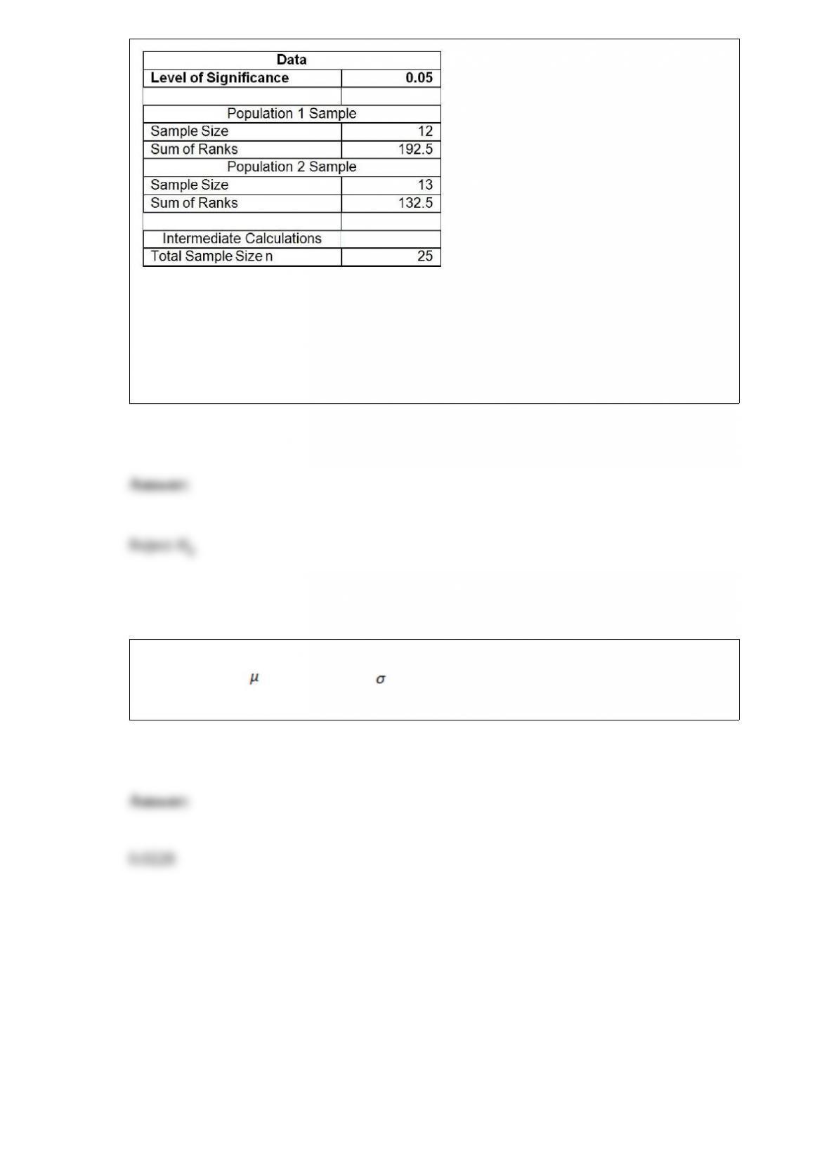
You are told that the gas mileage population distributions for both models are not
normally distributed.
Referring to Table 12-15, what is your decision on the test using a 5% level of
significance?
The amount of tea leaves in a can from a particular production line is normally
distributed with = 110 grams and = 25 grams. A sample of 25 cans is to be selected.
What is the probability that the sample mean will be less than 100 grams?