True or False: In testing a hypothesis, you should always raise the question concerning
the purpose of the study, survey or experiment.
True or False: If the values of the seventh and eighth class in a cumulative percentage
distribution are the same, we know that there are no observations in the eighth class.
True or False: TABLE 18-5
A manufacturer of computer disks took samples of 240 disks on 15 consecutive days.
The number of disks with bad sectors was determined for each of these samples. The
results are in the table that follows.
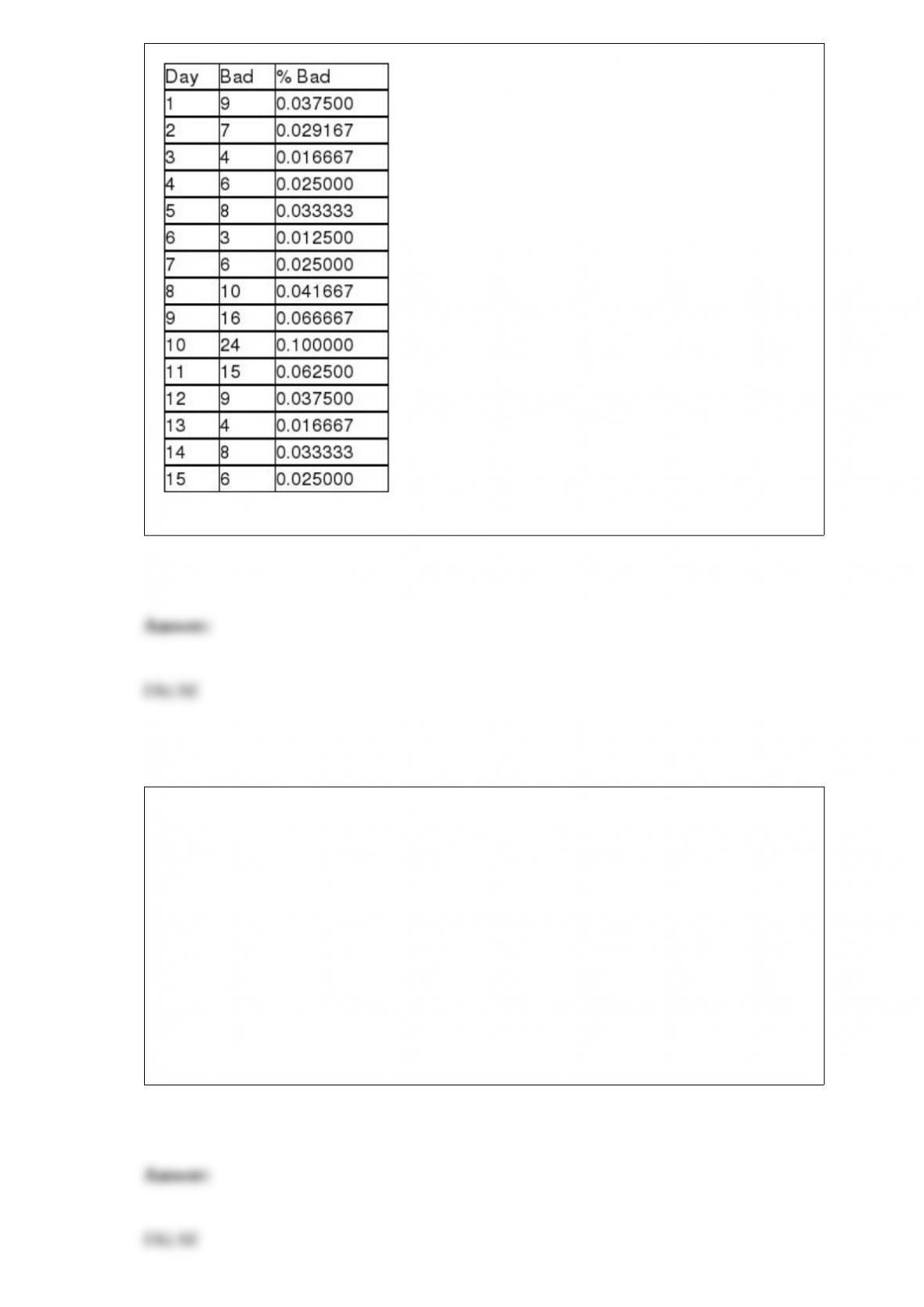
Referring to Table 18-5, the process seems to be in control.
TABLE 12-2
The dean of a college is interested in the proportion of graduates from his college who
have a job offer on graduation day. He is particularly interested in seeing if there is a
difference in this proportion for accounting and economics majors. In a random sample
of 100 of each type of major at graduation, he found that 65 accounting majors and 52
economics majors had job offers. If the accounting majors are designated as “Group 1”
and the economics majors are designated as “Group 2,” perform the appropriate
hypothesis test using a level of significance of 0.05.
True or False: Referring to Table 12-2, the same decision would be made with this test
if the level of significance had been 0.10 rather than 0.05.

True or False: A sample is used to obtain a 95% confidence interval for the mean of a
population. The confidence interval goes from 15 to 19. If the same sample had been
used to test the null hypothesis that the mean of the population is equal to 20 versus the
alternative hypothesis that the mean of the population differs from 20, the null
hypothesis could be rejected at a level of significance of 0.10.
True or False: The F test in a completely randomized model is just an expansion of the t
test for independent samples.
True or False: TABLE 17-9
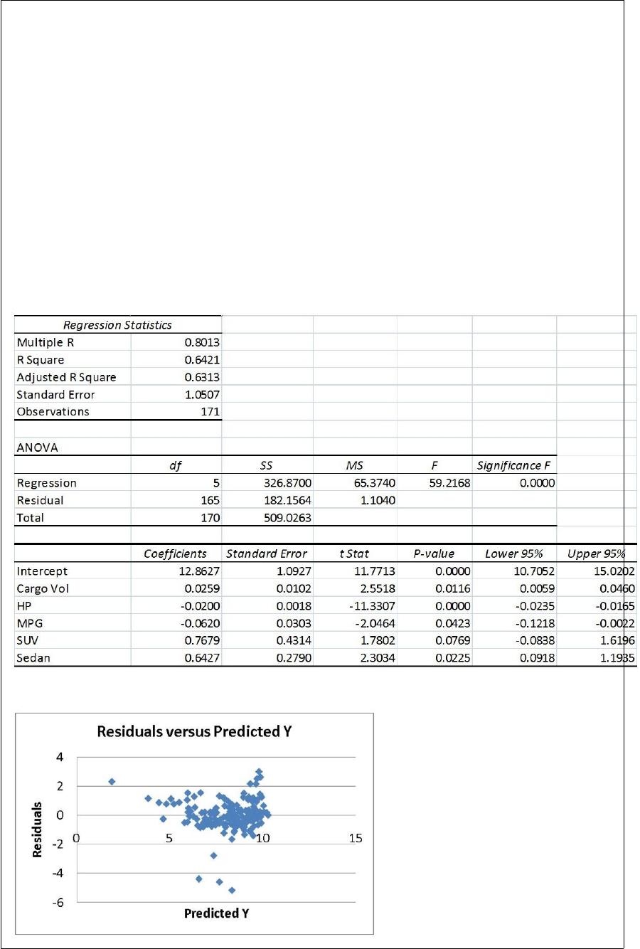
What are the factors that determine the acceleration time (in sec.) from 0 to 60 miles per
hour of a car? Data on the following variables for 171 different vehicle models were
collected:
Accel Time: Acceleration time in sec.
Cargo Vol: Cargo volume in cu. ft.
HP: Horsepower
MPG: Miles per gallon
SUV: 1 if the vehicle model is an SUV with Coupe as the base when SUV and Sedan
are both 0
Sedan: 1 if the vehicle model is a sedan with Coupe as the base when SUV and Sedan
are both 0
The regression results using acceleration time as the dependent variable and the
remaining variables as the independent variables are presented below.
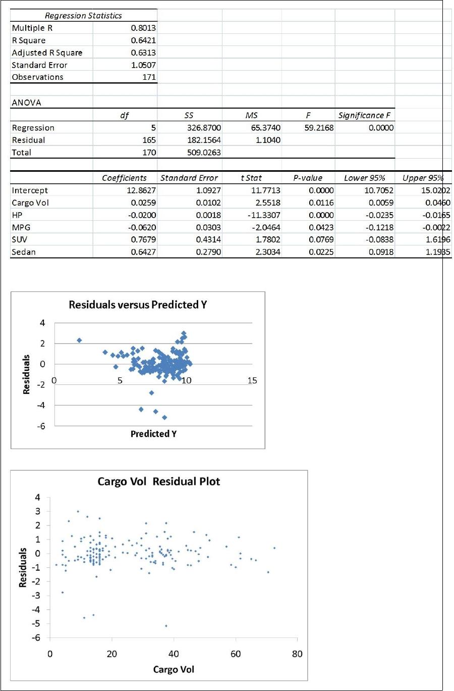
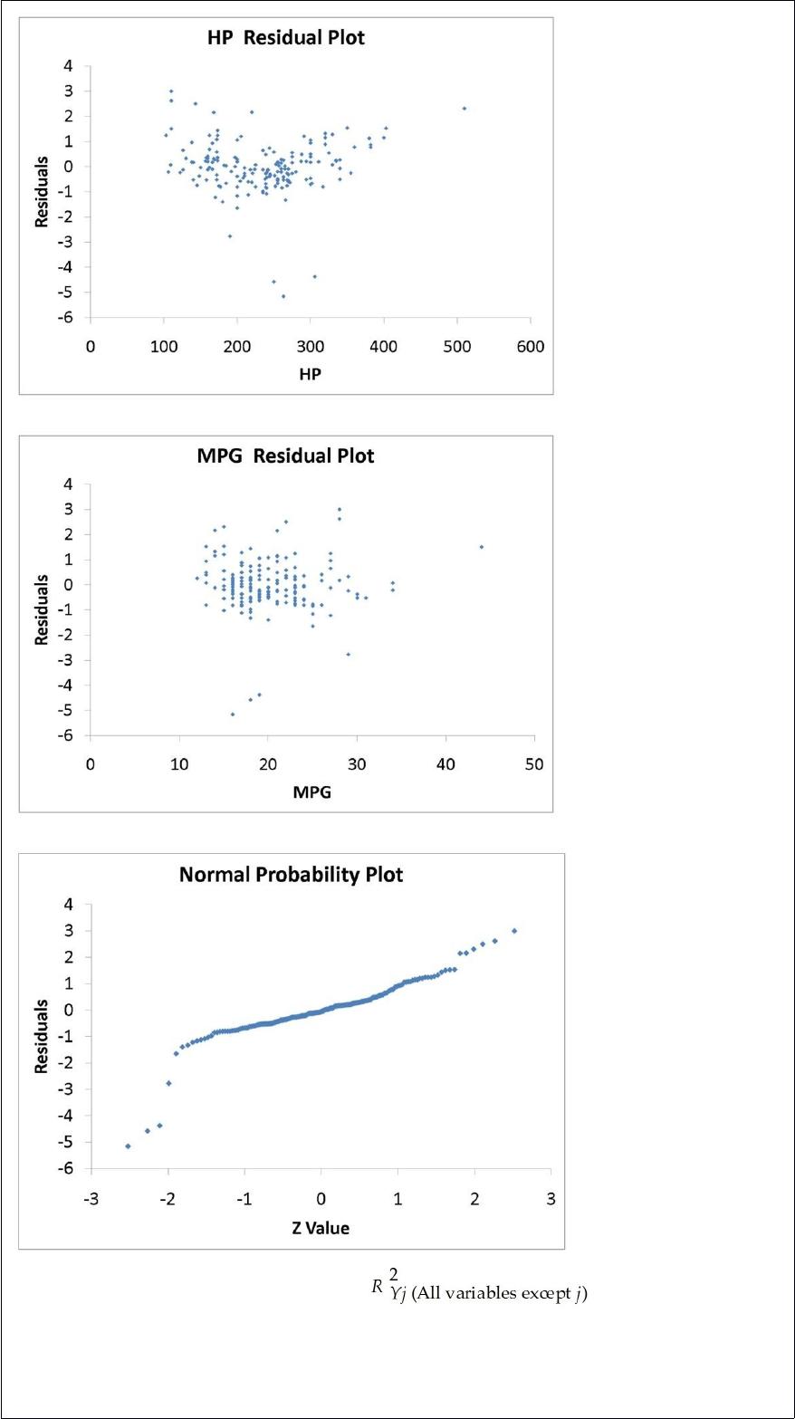
The various residual plots are as shown below.
The coefficient of partial determination ( ) of each of the 5
predictors are, respectively, 0.0380, 0.4376, 0.0248, 0.0188, and 0.0312.
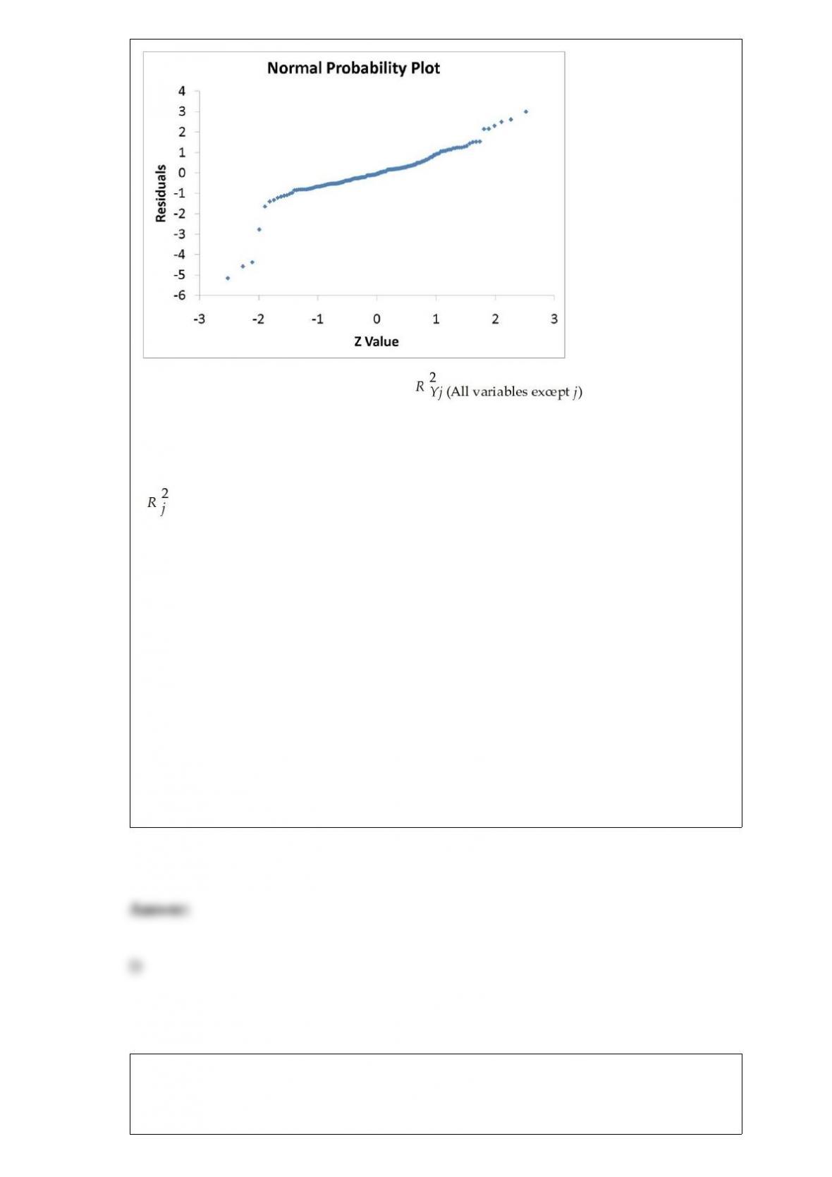
The coefficient of multiple determination for the regression model using each of the 5
variables Xj as the dependent variable and all other X variables as independent variables
( ) are, respectively, 0.7461, 0.5676, 0.6764, 0.8582, 0.6632.
Referring to Table 17-9, the 0 to 60 miles per hour acceleration time of an SUV is
predicted to be 0.1252 seconds higher than that of a sedan.
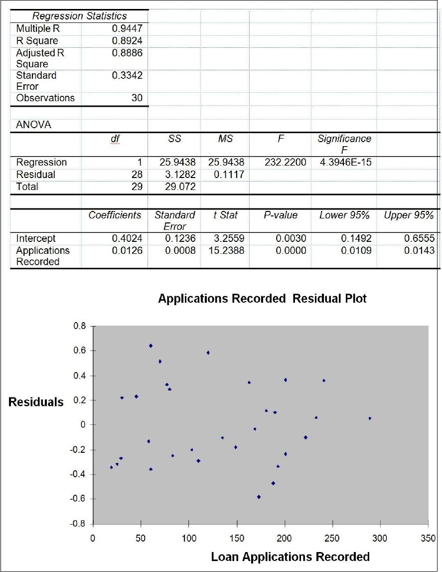
TABLE 11-11
A student team in a business statistics course designed an experiment to investigate
whether the brand of bubblegum used affected the size of bubbles they could blow. To
reduce the person-to-person variability, the students decided to use a randomized block
design using themselves as blocks.
Four brands of bubblegum were tested. A student chewed two pieces of a brand of gum
and then blew a bubble, attempting to make it as big as possible. Another student
measured the diameter of the bubble at its biggest point. The following table gives the
diameters of the bubbles (in inches) for the 16 observations.
True or False: Referring to Table 11-11, the randomized block F test is valid only if the
population of diameters has the same variance for the 4 brands.
True or False: An investment consultant is recommending a certain class of mutual
funds to the clienteles based on its exceptionally high probability of gain. It is an ethical
practice to explain to the clienteles what the meaning of probability is.

True or False: Referring to Table 14-16, the 0 to 60 miles per hour
acceleration time of a sedan is predicted to be 0.0005 seconds lower
than that of a non-sedan with the same engine size.
TABLE 13-12
The manager of the purchasing department of a large saving and loan organization
would like to develop a model to predict the amount of time (measured in hours) it
takes to record a loan application. Data are collected from a sample of 30 days, and the
number of applications recorded and completion time in hours is recorded. Below is the
regression output:
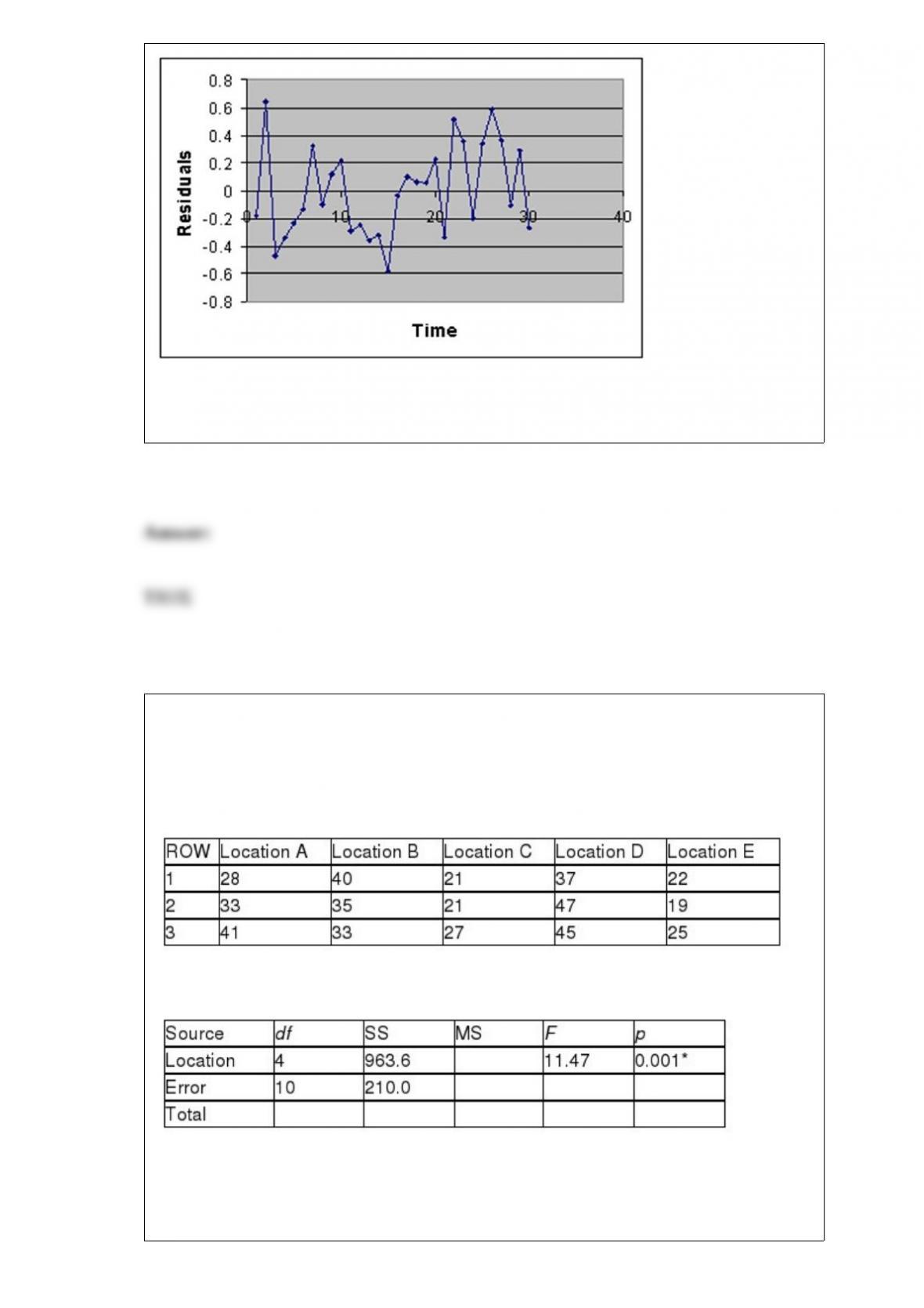
True or False: Referring to Table 13-12, the model appears to be adequate based on the
residual analyses.
TABLE 11-5
A hotel chain has identically small sized resorts in 5 locations in different small islands.
The data that follow resulted from analyzing the hotel occupancies on randomly
selected days in the 5 locations.
Analysis of Variance
* or p < 0.005, tabular value
True or False: Referring to Table 11-5, if a level of significance of 0.05 is chosen, the
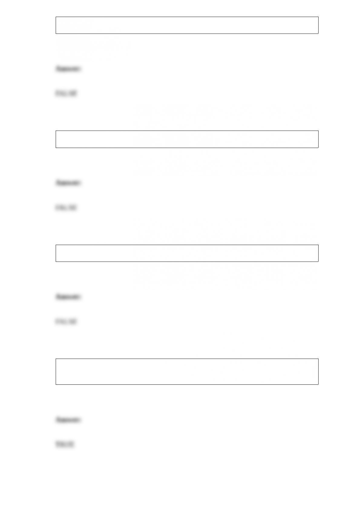
decision made indicates that all 5 locations have different mean occupancy rates.
True or False: A polygon can be constructed from a bar chart.
True or False: The purpose of a control chart is to eliminate common cause variation.
True or False: A test for the difference between two proportions can be performed using
the chi-square distribution.
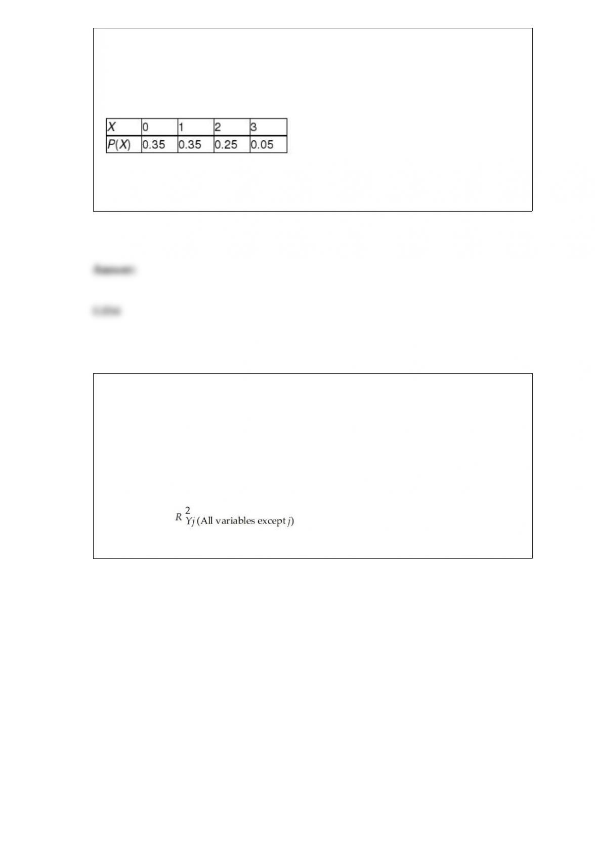
TABLE 5-3
The following table contains the probability distribution for X = the number of
retransmissions necessary to successfully transmit a 1024K data package through a
double satellite media.
Referring to Table 5-3, the standard deviation of the number of retransmissions is
________.
TABLE 17-10
Given below are results from the regression analysis where the dependent variable is
the number of weeks a worker is unemployed due to a layoff (Unemploy) and the
independent variables are the age of the worker (Age), the number of years of education
received (Edu), the number of years at the previous job (Job Yr), a dummy variable for
marital status (Married: 1 = married, 0 = otherwise), a dummy variable for head of
household (Head: 1 = yes, 0 = no) and a dummy variable for management position
(Manager: 1 = yes, 0 = no). We shall call this Model 1. The coefficient of partial
determination ( ) of each of the 6 predictors are, respectively,
0.2807, 0.0386, 0.0317, 0.0141, 0.0958, and 0.1201.
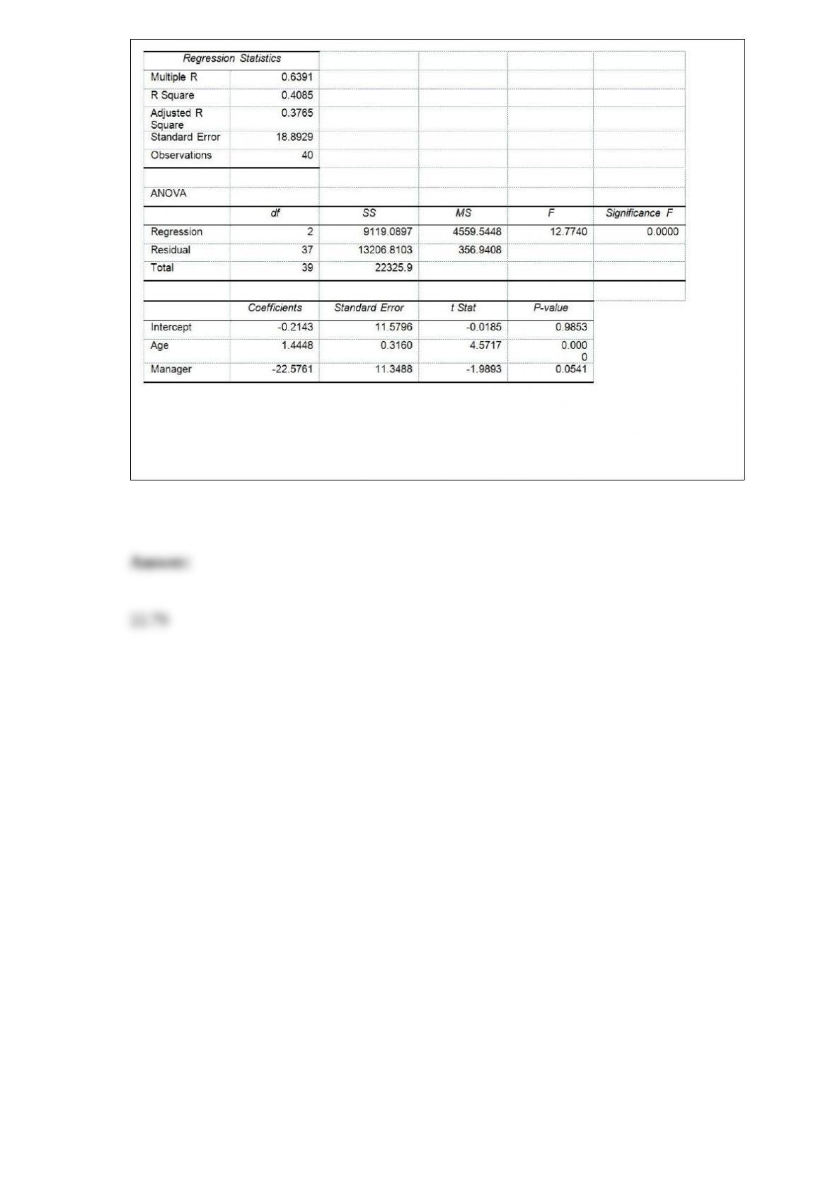
Model 2 is the regression analysis where the dependent variable is Unemploy and the
independent variables are Age and Manager. The results of the regression analysis are
given below:
Referring to Table 17-10, Model 1, which of the following is the correct alternative
hypothesis to determine whether there is a significant relationship between the number
of weeks a worker is unemployed due to a layoff and the entire set of explanatory
variables?
A) H1 : All βj ≠0 for j = 0, 1, 2, 3, 4, 5, 6
B) H1 : All βj ≠0 for j = 1, 2, 3, 4, 5, 6
C) H1 : At least one of βj ≠0 for j = 0, 1, 2, 3, 4, 5, 6
D) H1 : At least one of βj ≠0 for j = 1, 2, 3, 4, 5, 6
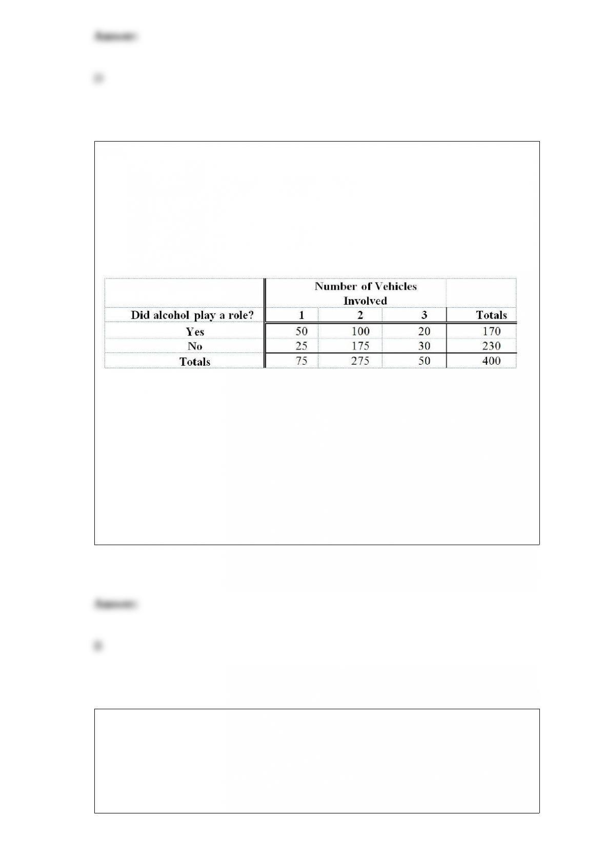
TABLE 4-1
Mothers Against Drunk Driving is a very visible group whose main focus is to educate
the public about the harm caused by drunk drivers. A study was recently done that
emphasized the problem we all face with drinking and driving. Four hundred accidents
that occurred on a Saturday night were analyzed. Two items noted were the number of
vehicles involved and whether alcohol played a role in the accident. The numbers are
shown below:
Referring to Table 4-1, given alcohol was involved, what proportion of accidents
involved a single vehicle?
A) 50/75 or 66.67%
B) 50/170 or 29.41%
C) 120/170 or 70.59%
D) 120/400 or 30%
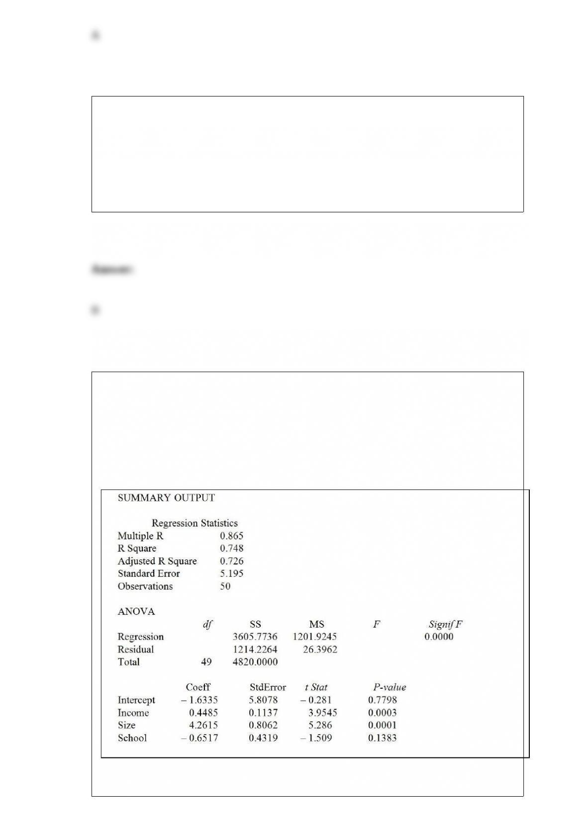
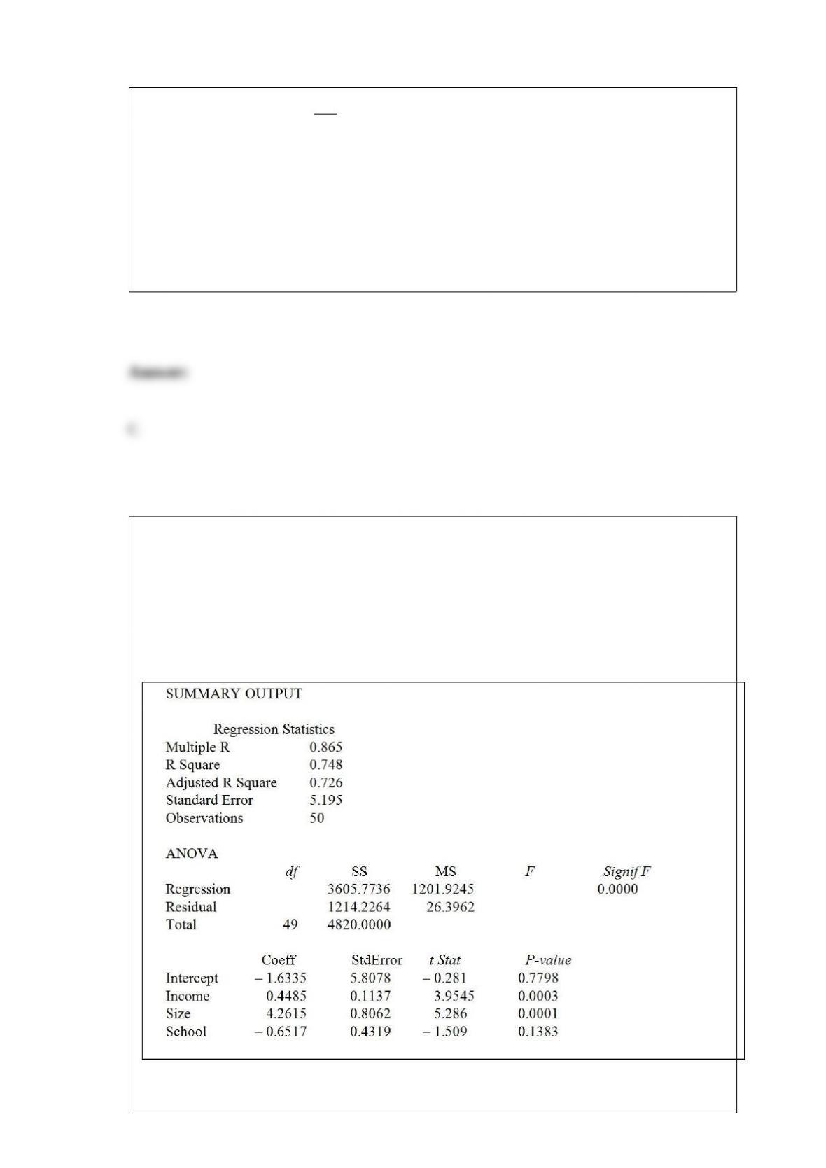
TABLE 17-1
A real estate builder wishes to determine how house size (House) is influenced by
family income (Income), family size (Size), and education of the head of household
(School). House size is measured in hundreds of square feet, income is measured in
thousands of dollars, and education is in years. The builder randomly selected 50
families and ran the multiple regression. Microsoft Excel output is provided below:
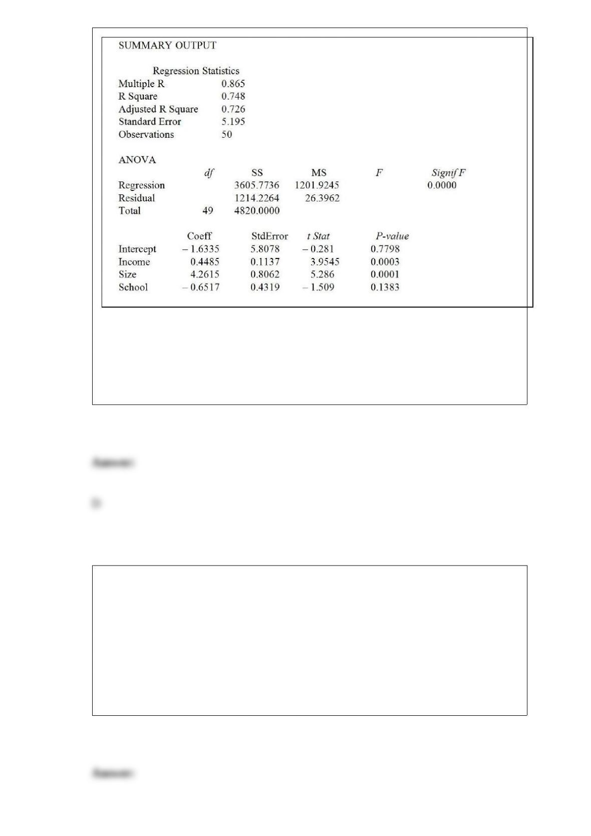
Referring to Table 17-1, what is the value of the calculated F test statistic that is
missing from the output for testing whether the whole regression model is significant?
A) 0.0001
B) 0.0299
C) 0.726
D) 45.5340
The Y-intercept (b0) represents the
A) estimated average Y when X = 0.
B) change in estimated average Y per unit change in X.
C) predicted value of Y.
D) variation around the sample regression line.
The principal focus of the control chart is the attempt to separate special or assignable
causes of variation from common causes of variation. Which causes of variation can be
reduced only by changing the system?
A) Special or assignable causes
B) Common causes
C) Total causes
D) None of the above
TABLE 17-1
A real estate builder wishes to determine how house size (House) is influenced by
family income (Income), family size (Size), and education of the head of household
(School). House size is measured in hundreds of square feet, income is measured in
thousands of dollars, and education is in years. The builder randomly selected 50
families and ran the multiple regression. Microsoft Excel output is provided below:
Referring to Table 17-1, suppose the builder wants to test whether the coefficient on
Income is significantly different from 0. What is the value of the relevant t-statistic?
A) 5.286
B) 5.195
C) 3.945
D) -1.509
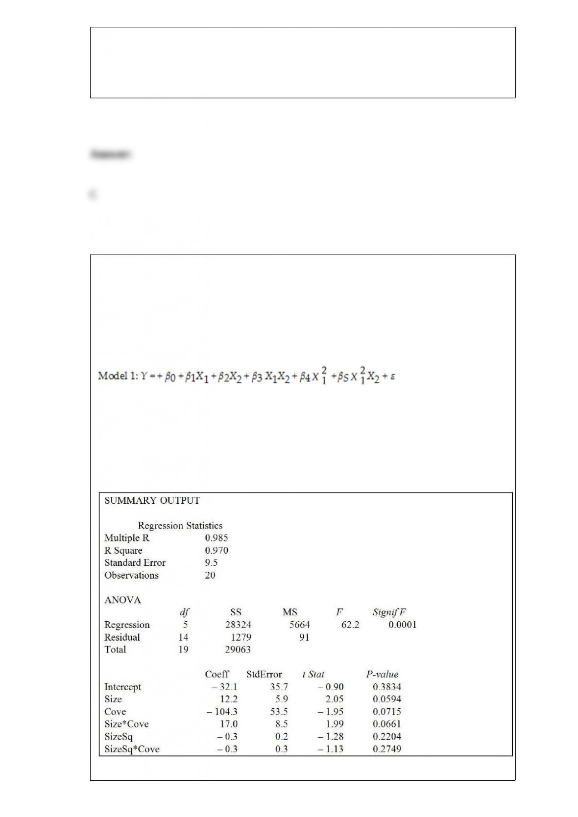
TABLE 15-2
In Hawaii, condemnation proceedings are under way to enable private citizens to own
the property that their homes are built on. Until recently, only estates were permitted to
own land, and homeowners leased the land from the estate. In order to comply with the
new law, a large Hawaiian estate wants to use regression analysis to estimate the fair
market value of the land. The following model was fit to data collected for n = 20
properties, 10 of which are located near a cove.
where Y = Sale price of property in thousands of dollars
X1 = Size of property in thousands of square feet
X2 = 1 if property located near cove, 0 if not
Using the data collected for the 20 properties, the following partial output obtained
from Microsoft Excel is shown:
Referring to Table 15-2, is the overall model statistically adequate at a 0.05 level of
significance for predicting sale price (Y)?
A) No, since some of the t tests for the individual variables are not significant.
B) No, since the standard deviation of the model is fairly large.
C) Yes, since none of the -estimates are equal to 0.
D) Yes, since the p-value for the test is smaller than 0.05.
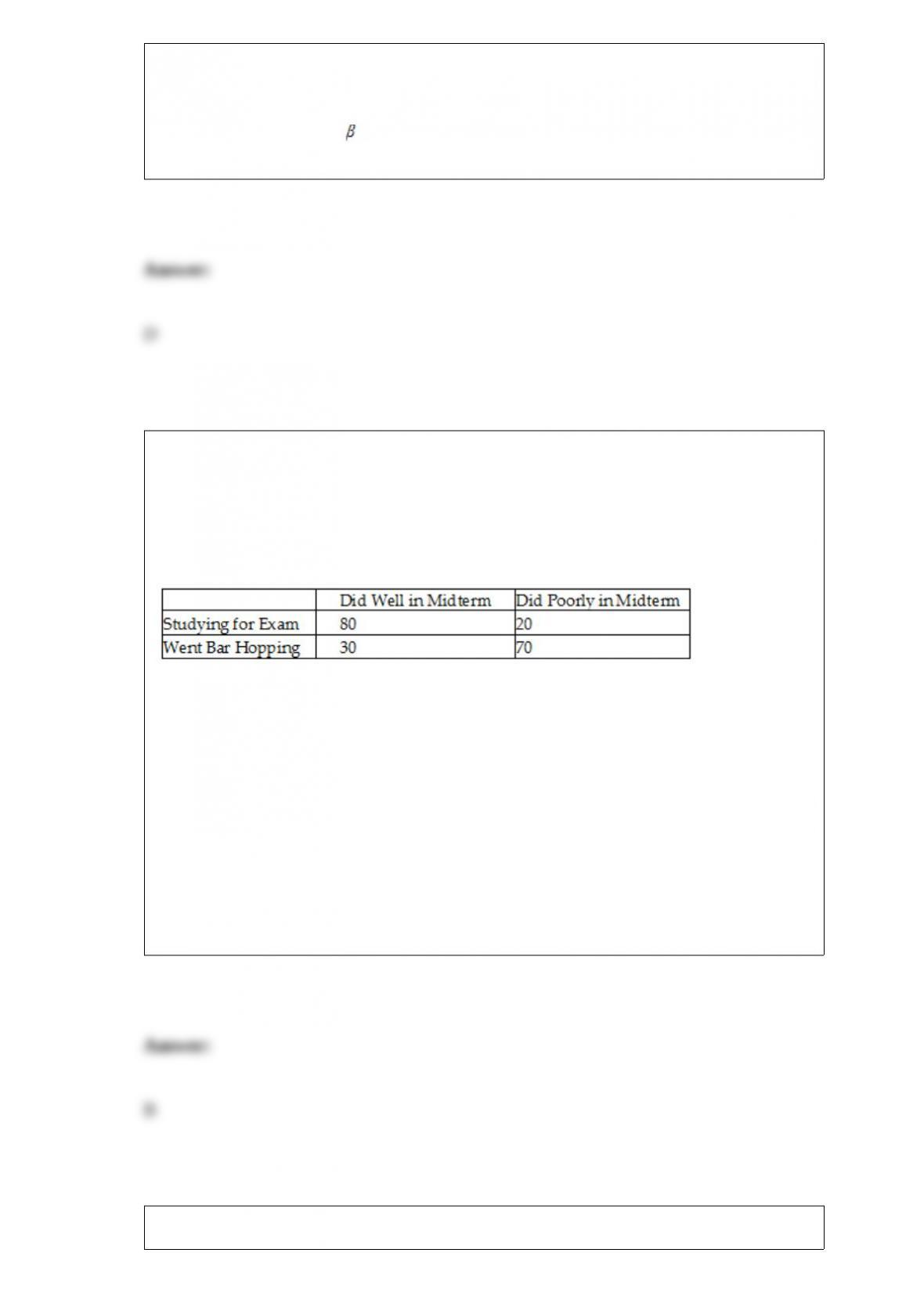
TABLE 2-6
A sample of 200 students at a Big-Ten university was taken after the midterm to ask
them whether they went bar hopping the weekend before the midterm or spent the
weekend studying, and whether they did well or poorly on the midterm. The following
table contains the result.
Referring to Table 2-6, if the sample is a good representation of the population, we can
expect ________ percent of those who did poorly on the midterm to have spent the
weekend studying.
A) 10
B) 22
C) 45
D) 50
TABLE 17-9
What are the factors that determine the acceleration time (in sec.) from 0 to 60 miles per
hour of a car? Data on the following variables for 171 different vehicle models were
collected:
Accel Time: Acceleration time in sec.
Cargo Vol: Cargo volume in cu. ft.
HP: Horsepower
MPG: Miles per gallon
SUV: 1 if the vehicle model is an SUV with Coupe as the base when SUV and Sedan
are both 0
Sedan: 1 if the vehicle model is a sedan with Coupe as the base when SUV and Sedan
are both 0
The regression results using acceleration time as the dependent variable and the
remaining variables as the independent variables are presented below.
The various residual plots are as shown below.
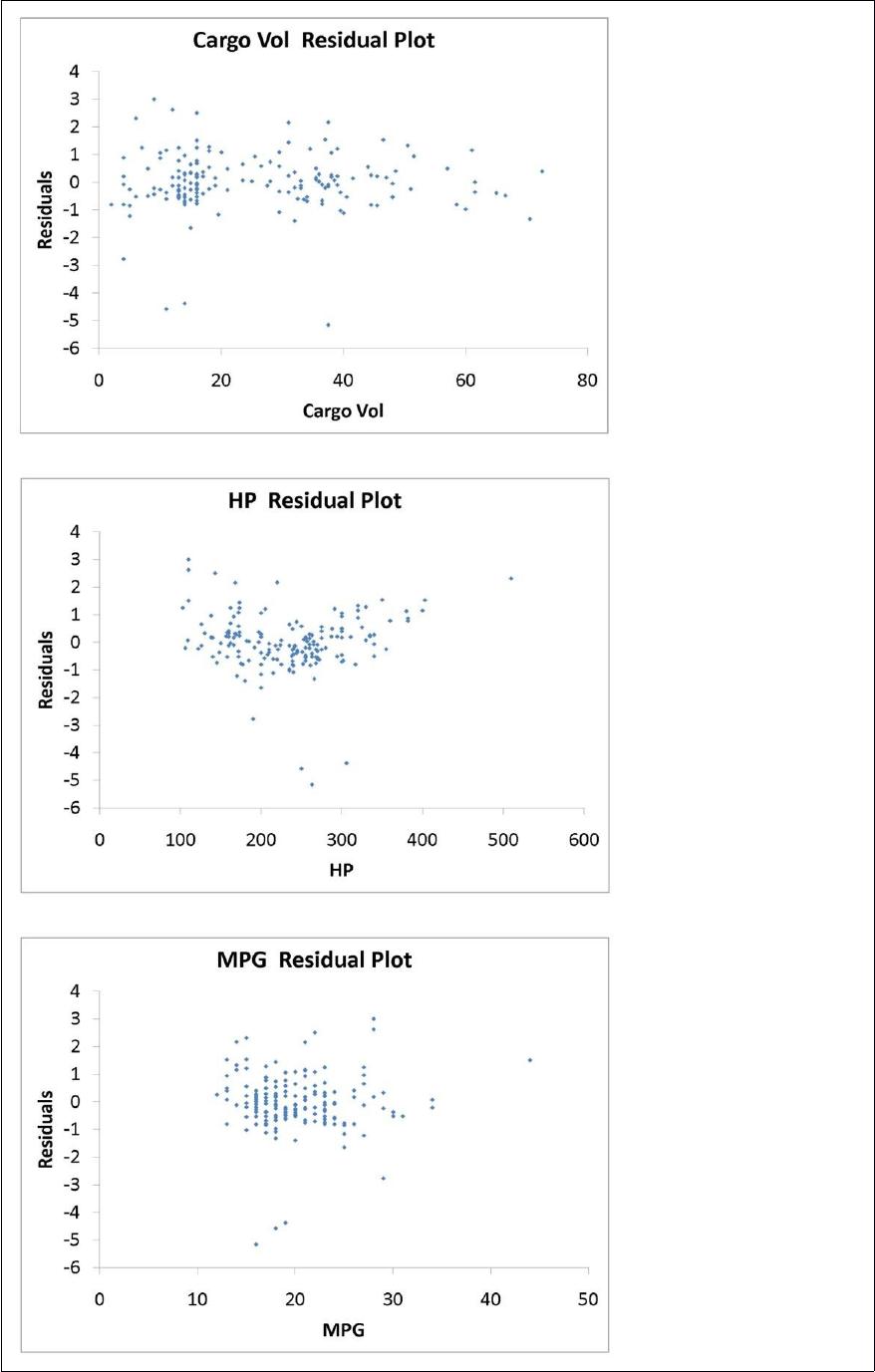
The coefficient of partial determination ( ) of each of the 5
predictors are, respectively, 0.0380, 0.4376, 0.0248, 0.0188, and 0.0312.
The coefficient of multiple determination for the regression model using each of the 5
variables Xj as the dependent variable and all other X variables as independent variables
( ) are, respectively, 0.7461, 0.5676, 0.6764, 0.8582, 0.6632.
Referring to Table 17-9, what is the correct interpretation for the estimated coefficient
for Cargo Vol?
A) As the 0 to 60 miles per hour acceleration time increases by one second, the mean
cargo volume will increase by an estimated 0.0259 cubic foot without taking into
consideration all the other independent variables included in the model.
B) As the cargo volume increases by one cubic foot, the mean 0 to 60 miles per hour
acceleration time will increase by an estimated 0.0259 seconds without taking into
consideration all the other independent variables included in the model.
C) As the 0 to 60 miles per hour acceleration time increases by one second, the mean
cargo volume will increase by an estimated 0.0259 cubic foot taking into consideration
all the other independent variables included in the model.
D) As the cargo volume increases by one cubic foot, the mean 0 to 60 miles per hour
acceleration time will increase by an estimated 0.0259 seconds taking into
consideration all the other independent variables included in the model.
The estimation of the population average family expenditure on food based on the
sample average expenditure of 1,000 families is an example of
A) inferential statistics.
B) descriptive statistics.
C) DCOVA framework.
D) operational definition.
TABLE 17-12
The marketing manager for a nationally franchised lawn service company would like to
study the characteristics that differentiate home owners who do and do not have a lawn
service. A random sample of 30 home owners located in a suburban area near a large
city was selected; 15 did not have a lawn service (code 0) and 15 had a lawn service
(code 1). Additional information available concerning these 30 home owners includes
family income (Income, in thousands of dollars), lawn size (Lawn Size, in thousands of
square feet), attitude toward outdoor recreational activities (Attitude 0 = unfavorable, 1
= favorable), number of teenagers in the household (Teenager), and age of the head of
the household (Age).
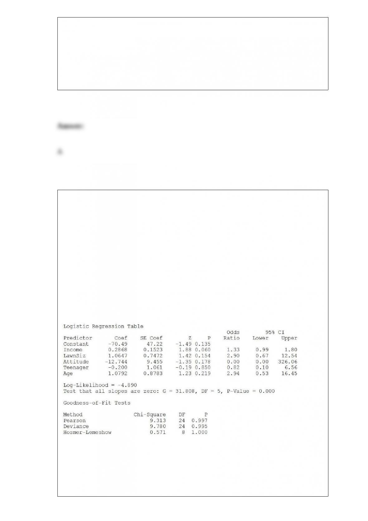
The Minitab output is given below:
Referring to Table 17-12, which of the following is the correct interpretation for the
Income slope coefficient?
A) Holding constant the effect of the other variables, the estimated number of lawn
services purchased increases by 0.2868 for each increase of one thousand dollars in

family income.
B) Holding constant the effect of the other variables, the estimated average number of
lawn services purchased increases by 0.2868 for each increase of one thousand dollars
in family income.
C) Holding constant the effect of the other variables, the estimated probability of
purchasing a lawn service increases by 0.2868 for each increase of one thousand dollars
in family income.
D) Holding constant the effect of the other variables, the estimated natural logarithm of
the odds ratio of purchasing a lawn service increases by 0.2868 for each increase of one
thousand dollars in family income.
The Kruskal-Wallis test is an extension of which of the following for two independent
samples?
A) Pooled-variance t test
B) Paired-sample t test
C) Wilcoxon rank sum test
D) McNemar test
TABLE 19-2
The following payoff matrix is given in dollars.
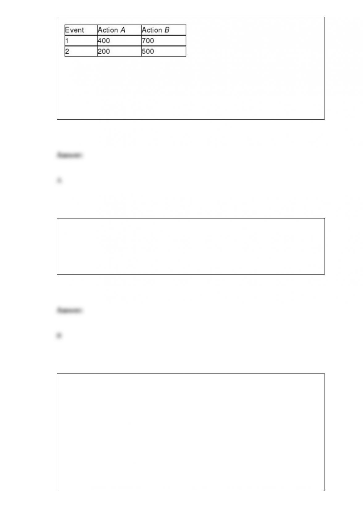
Suppose the probability of Event 1 is 0.5 and Event 2 is 0.5.
Referring to Table 19-2, the EMV for Action A is
A) $300.
B) $550.
C) $600.
D) $700.
Which of the following is used to find a “best” model?
A) Odds ratio
B) Mallow’s Cp
C) Standard error of the estimate
D) SST
TABLE 11-8
A physician and president of a Tampa Health Maintenance Organization (HMO) are
attempting to show the benefits of managed health care to an insurance company. The
physician believes that certain types of doctors are more cost-effective than others. One
theory is that Primary Specialty is an important factor in measuring the
cost-effectiveness of physicians. To investigate this, the president obtained independent
random samples of 20 HMO physicians from each of 4 primary specialties – General
Practice (GP), Internal Medicine (IM), Pediatrics (PED), and Family Physicians (FP) –
and recorded the total charges per member per month for each. A second factor which
the president believes influences total charges per member per month is whether the
doctor is a foreign or USA medical school graduate. The president theorizes that foreign
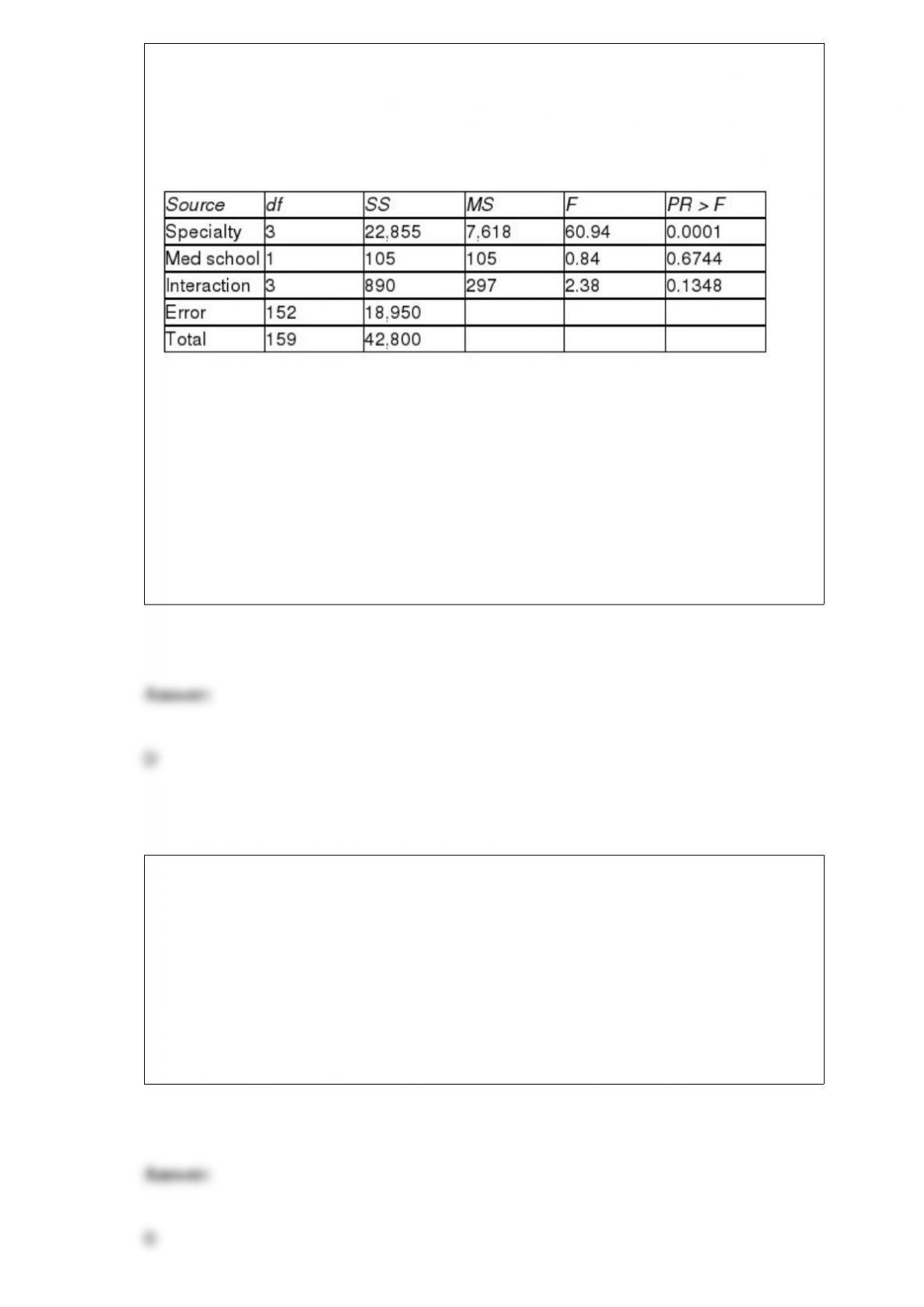
graduates will have higher mean charges than USA graduates. To investigate this, the
president also collected data on 20 foreign medical school graduates in each of the 4
primary specialty types described above. So information on charges for 40 doctors (20
foreign and 20 USA medical school graduates) was obtained for each of the 4
specialties. The results for the ANOVA are summarized in the following table.
Referring to Table 11-8, what was the total number of doctors included in the study?
A) 20
B) 40
C) 159
D) 160
Blossom’s Flowers purchases roses for sale for Valentine’s Day. The roses are purchased
for $10 a dozen and are sold for $20 a dozen. Any roses not sold on Valentine’s Day can
be sold for $5 per dozen. The owner will purchase 1 of 3 amounts of roses for
Valentine’s Day: 100, 200, or 400 dozen roses. The opportunity loss for buying 200
dozen roses and selling 100 dozen roses at the full price is
A) $1,000.
B) $500.
C) -$500.
D) -$2,000.
Which of the following is not a reason for selecting a sample?
A) A sample is less time consuming than a census.
B) A sample is less costly to administer than a census.
C) A sample is usually not a good representation of the target population.
D) A sample is less cumbersome and more practical to administer.
TABLE 17-1
A real estate builder wishes to determine how house size (House) is influenced by
family income (Income), family size (Size), and education of the head of household
(School). House size is measured in hundreds of square feet, income is measured in
thousands of dollars, and education is in years. The builder randomly selected 50
families and ran the multiple regression. Microsoft Excel output is provided below:
Referring to Table 17-1, one individual in the sample had an annual income of
$100,000, a family size of 10, and an education of 16 years. This individual owned a

home with an area of 7,000 square feet (House = 70.00). What is the residual (in
hundreds of square feet) for this data point?
A) 7.40
B) 2.52
C) -2.52
D) -5.40
Referring to Table 14-7, the net regression coefficient of X2 is ________.
TABLE 14-7
The department head of the accounting department wanted to see if
she could predict the GPA of students using the number of course
units (credits) and total SAT scores of each. She takes a sample of
students and generates the following Microsoft Excel output:
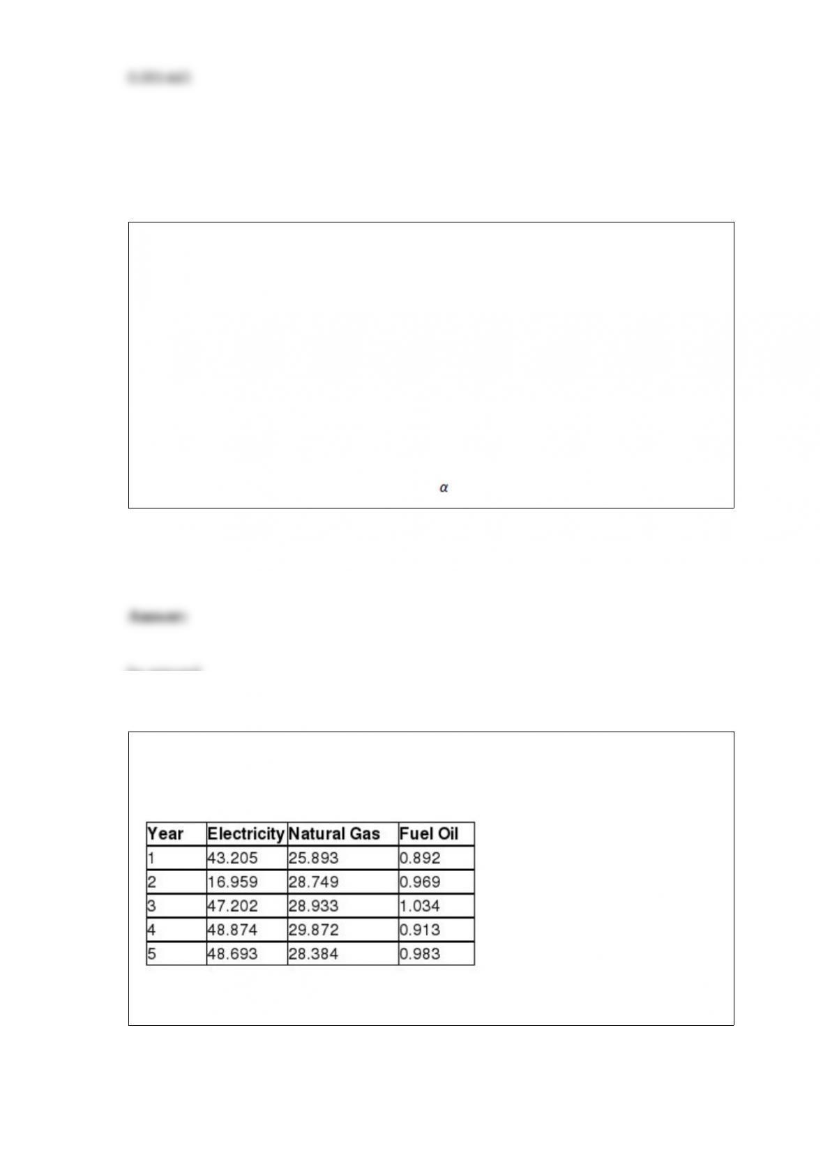
TABLE 10-6
To investigate the efficacy of a diet, a random sample of 16 male patients is selected
from a population of adult males using the diet. The weight of each individual in the
sample is taken at the start of the diet and at a medical follow-up 4 weeks later.
Assuming that the population of differences in weight before versus after the diet
follow a normal distribution, the t-test for related samples can be used to determine if
there was a significant decrease in the mean weight during this period. Suppose the
mean decrease in weights over all 16 subjects in the study is 3.0 pounds with the
standard deviation of differences computed as 6.0 pounds.
Referring to Table 10-6, a one-tail test of the null hypothesis of no difference would
________ (be rejected/not be rejected) at the = 0.05 level of significance.
TABLE 16-15
Given below are the average prices for three types of energy products for five
consecutive years.
Referring to Table 16-15, what is the unweighted aggregate price index for the group of
three energy items in year 3 using year 1 as the base year?

You were told that the mean score on a statistics exam is 75 with the scores normally
distributed. In addition, you know the probability of a score between 55 and 60 is
4.41% and that the probability of a score greater than 90 is 6.68%. What is the
probability of a score between 55 and 90?
If a researcher does not reject a true null hypothesis, she has made a(n) ________
decision.
TABLE 3-3
The ordered array below represents the number of vitamin supplements sold by a health
food store in a sample of 16 days.
19, 19, 20, 20, 22, 23, 25, 26, 27, 30, 33, 34, 35, 36, 38, 41
Note: For this sample, the sum of the values is 448, and the sum of the squared
differences between each value and the mean is 812.
Referring to Table 3-3, construct a boxplot for the data in this sample.
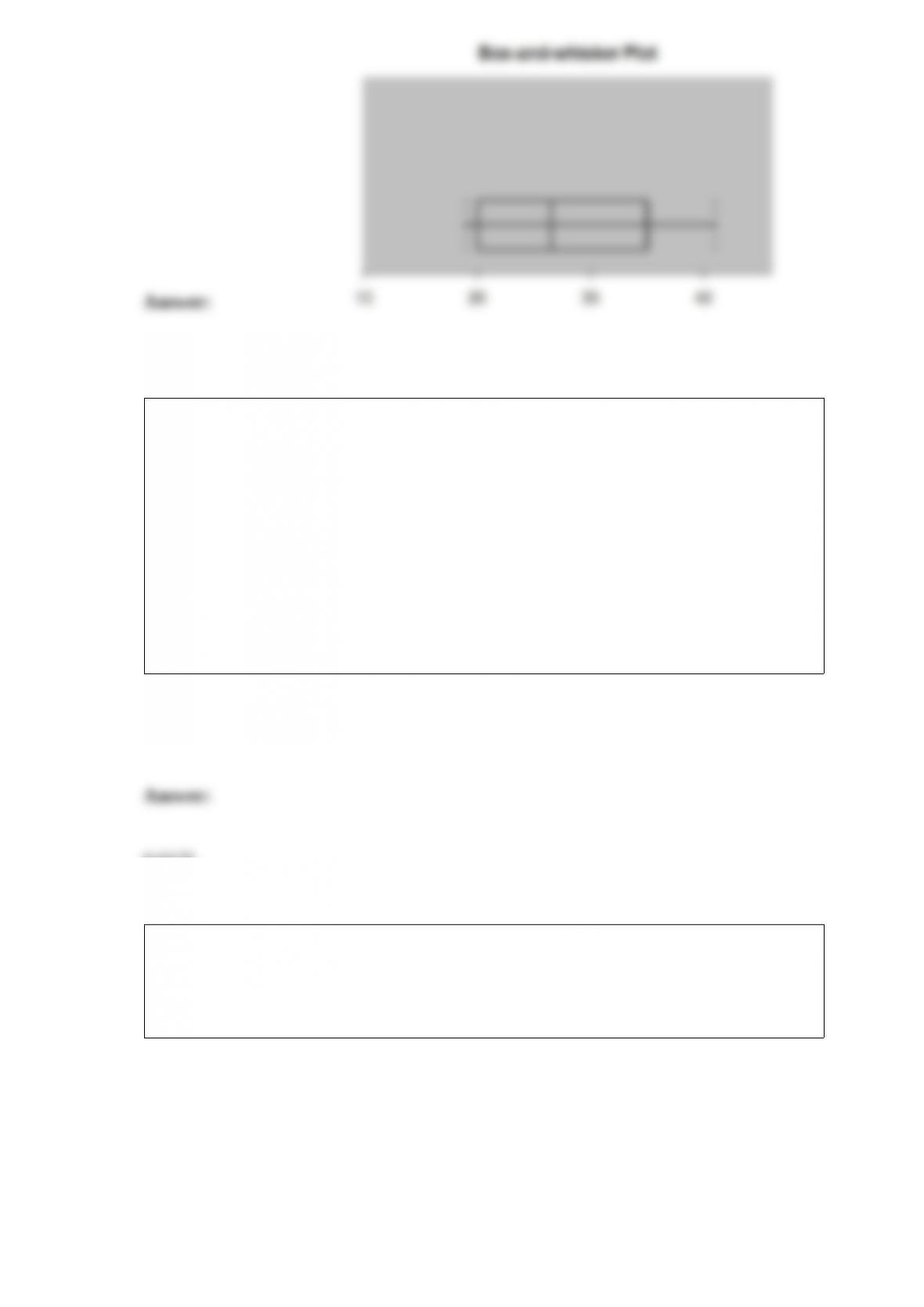
TABLE 9-11
An appliance manufacturer claims to have developed a compact microwave oven that
consumes a population mean of no more than 250 W. From previous studies, it is
believed that power consumption for microwave ovens is normally distributed with a
population standard deviation of 15 W. If there is evidence that the population mean
consumption is greater than 250 W, the manufacturer will be unable to make the claim.
Referring to Table 9-11, if you select a sample of 20 compact microwave ovens and are
willing to have a level of significance of 0.05, the power of the test is ________ if the
mean power consumption of all such microwave ovens is in fact 248 W.
TABLE 18-5
A manufacturer of computer disks took samples of 240 disks on 15 consecutive days.
The number of disks with bad sectors was determined for each of these samples. The
results are in the table that follows.
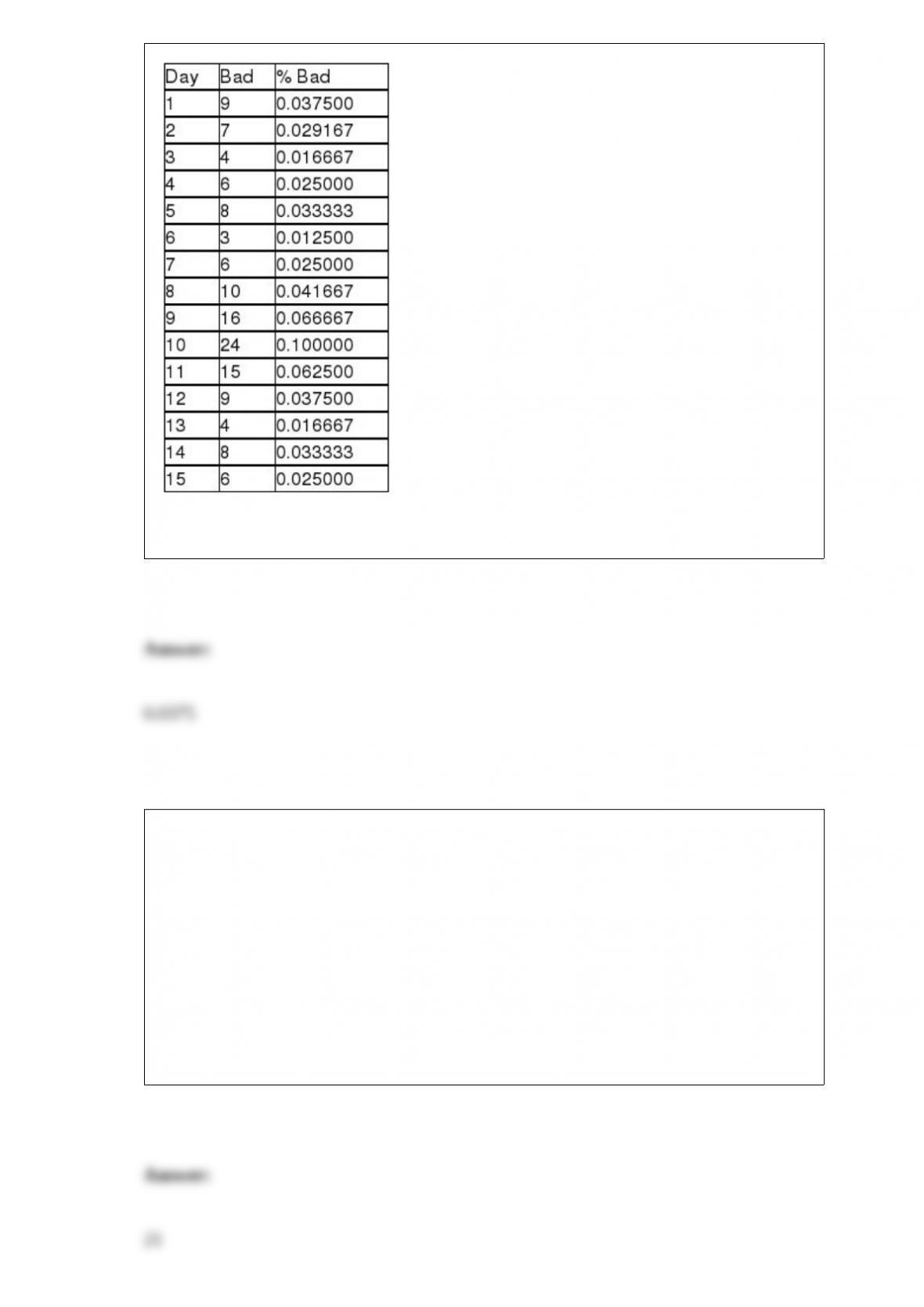
Referring to Table 18-5, the best estimate of the mean proportion of disks with bad
sectors is ________.
TABLE 3-4
The ordered array below represents the number of cargo manifests approved by customs
inspectors of the Port of New York in a sample of 35 days:
16, 17, 18, 18, 19, 20, 20, 21, 21, 21, 22, 22, 22, 22, 23, 23, 23, 23, 24, 24, 24, 25, 25,
26, 26, 26, 27, 28, 28, 29, 29, 31, 31, 32, 32
Note: For this sample, the sum of the values is 838, and the sum of the squared
differences between each value and the mean is 619.89.
Referring to Table 3-4, the first quartile of the customs data is ________.
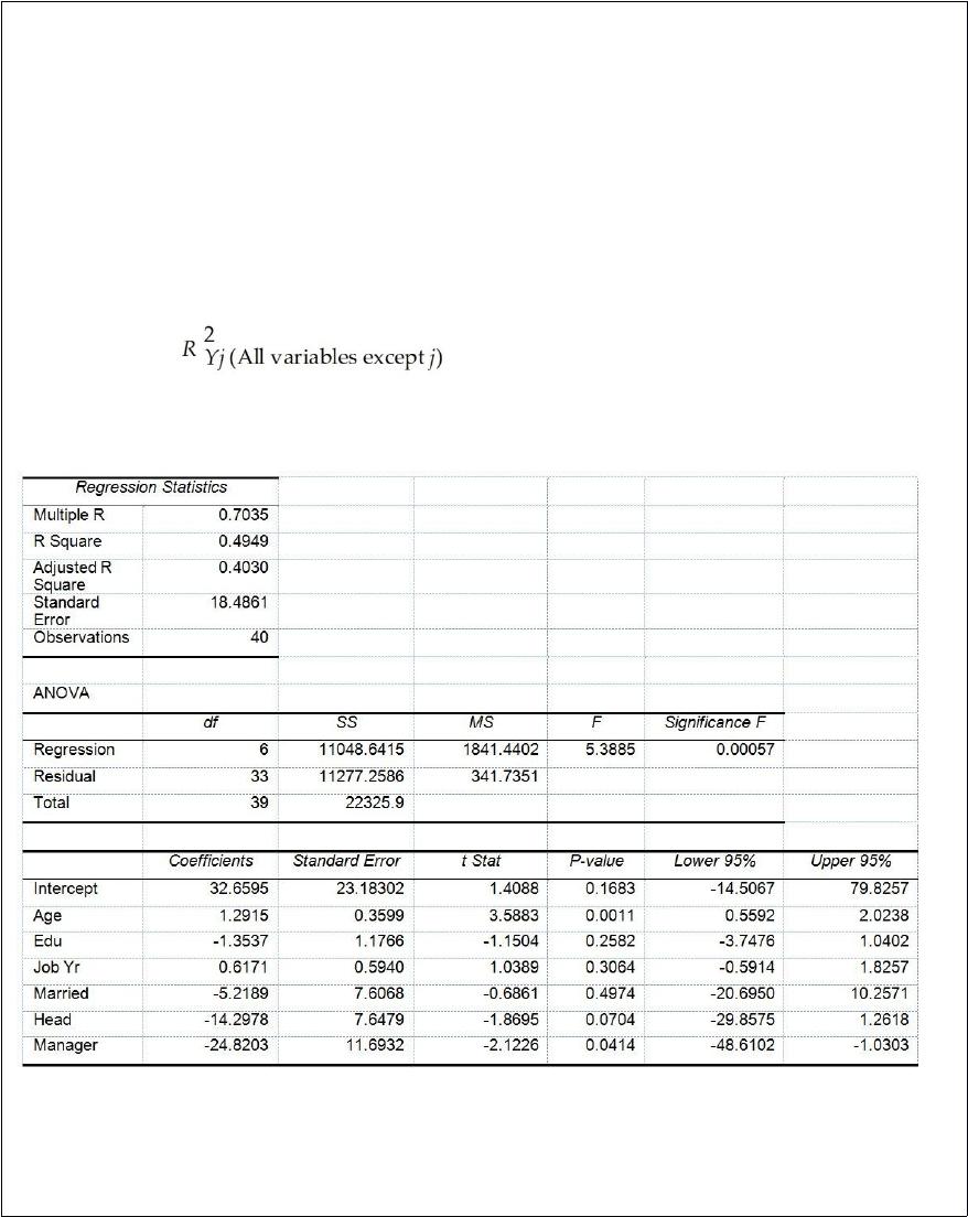
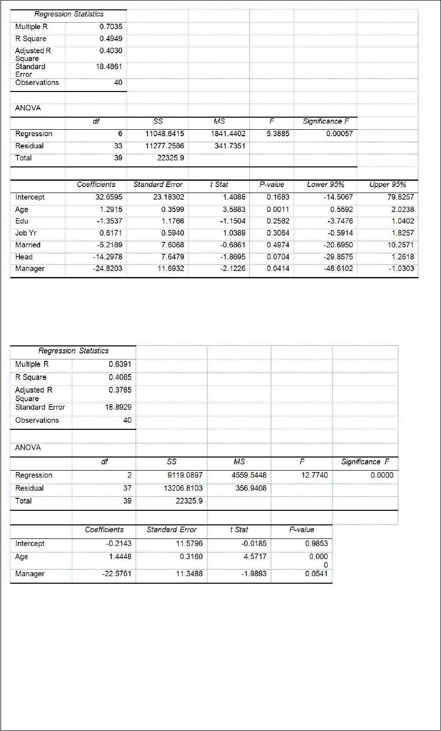
TABLE 17-10
Given below are results from the regression analysis where the dependent variable is
the number of weeks a worker is unemployed due to a layoff (Unemploy) and the
independent variables are the age of the worker (Age), the number of years of education
received (Edu), the number of years at the previous job (Job Yr), a dummy variable for
marital status (Married: 1 = married, 0 = otherwise), a dummy variable for head of
household (Head: 1 = yes, 0 = no) and a dummy variable for management position
(Manager: 1 = yes, 0 = no). We shall call this Model 1. The coefficient of partial
determination ( ) of each of the 6 predictors are, respectively,
0.2807, 0.0386, 0.0317, 0.0141, 0.0958, and 0.1201.
Model 2 is the regression analysis where the dependent variable is Unemploy and the
independent variables are Age and Manager. The results of the regression analysis are
given below:
Referring to Table 17-10, Model 1, predict the number of weeks being unemployed due
to a layoff for a worker who is a thirty-year-old, has 10 years of education, has 15 years
of experience at the previous job, is married, is the head of household and is a manager.