
TABLE 9-9
The president of a university claimed that the entering class this year appeared to be
larger than the entering class from previous years but their mean SAT score is lower
than previous years. He took a sample of 20 of this year’s entering students and found
that their mean SAT score is 1,501 with a standard deviation of 53. The university’s
record indicates that the mean SAT score for entering students from previous years is
1,520. He wants to find out if his claim is supported by the evidence at a 5% level of
significance.
True or False: Referring to Table 9-9, the president can conclude that there is sufficient
evidence to show that the mean SAT score of the entering class this year is lower than
previous years with no more than a 10% probability of incorrectly rejecting the true null
hypothesis.
True or False: The Variance Inflationary Factor (VIF) measures the correlation of the X
variables with the Y variable.
True or False: The probability that a standard normal variable, Z, is between 1.00 and
3.00 is 0.1574.
True or False: The McNemar test is used to determine whether there is evidence of a
difference between the proportions of two related samples.
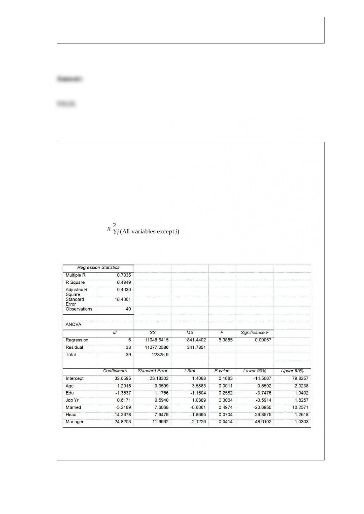
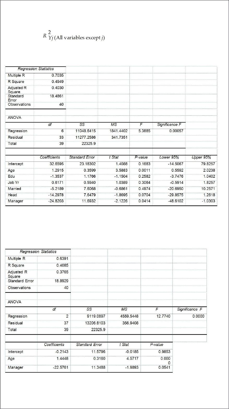
True or False: TABLE 17-10
Given below are results from the regression analysis where the dependent variable is
the number of weeks a worker is unemployed due to a layoff (Unemploy) and the
independent variables are the age of the worker (Age), the number of years of education
received (Edu), the number of years at the previous job (Job Yr), a dummy variable for
marital status (Married: 1 = married, 0 = otherwise), a dummy variable for head of
household (Head: 1 = yes, 0 = no) and a dummy variable for management position
(Manager: 1 = yes, 0 = no). We shall call this Model 1. The coefficient of partial
determination ( ) of each of the 6 predictors are, respectively,
0.2807, 0.0386, 0.0317, 0.0141, 0.0958, and 0.1201.
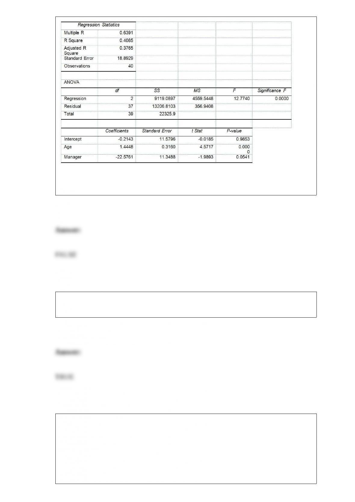
Model 2 is the regression analysis where the dependent variable is Unemploy and the
independent variables are Age and Manager. The results of the regression analysis are
given below:
Referring to Table 17-10, Model 1, there is sufficient evidence that the number of
weeks a worker is unemployed due to a layoff depends on all of the explanatory
variables at a 10% level of significance.
True or False: The CPL and CPU indexes are used to measure process’ actual
performance rather than its potential.
TABLE 6-2
John has two jobs. For daytime work at a jewelry store he is paid $15,000 per month,
plus a commission. His monthly commission is normally distributed with a mean of
$10,000 and a standard deviation of $2,000. At night he works occasionally as a waiter,
for which his monthly income is normally distributed with a mean of $1,000 and a
standard deviation of $300. John’s income levels from these two sources are
independent of each other.
Referring to Table 6-2, for a given month, what is the probability that John’s
commission from the jewelry store is more than $9,500?
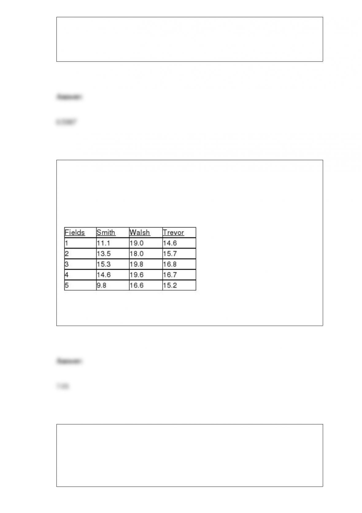
TABLE 11-10
An agronomist wants to compare the crop yield of 3 varieties of chickpea seeds. She
plants all 3 varieties of the seeds on each of 5 different patches of fields. She then
measures the crop yield in bushels per acre. Treating this as a randomized block design,
the results are presented in the table that follows.
Referring to Table 11-10, what is the critical value for testing the block effects at a 0.01
level of significance?
TABLE 17-10
Given below are results from the regression analysis where the dependent variable is
the number of weeks a worker is unemployed due to a layoff (Unemploy) and the
independent variables are the age of the worker (Age), the number of years of education
received (Edu), the number of years at the previous job (Job Yr), a dummy variable for
marital status (Married: 1 = married, 0 = otherwise), a dummy variable for head of
household (Head: 1 = yes, 0 = no) and a dummy variable for management position
(Manager: 1 = yes, 0 = no). We shall call this Model 1. The coefficient of partial
determination ( ) of each of the 6 predictors are, respectively,
0.2807, 0.0386, 0.0317, 0.0141, 0.0958, and 0.1201.
Model 2 is the regression analysis where the dependent variable is Unemploy and the
independent variables are Age and Manager. The results of the regression analysis are
given below:
Referring to Table 17-10, Model 1, estimate the mean number of weeks being
unemployed due to a layoff for a worker who is a thirty-year-old, has 10 years of
education, has 15 years of experience at the previous job, is married, is the head of
household and is a manager.
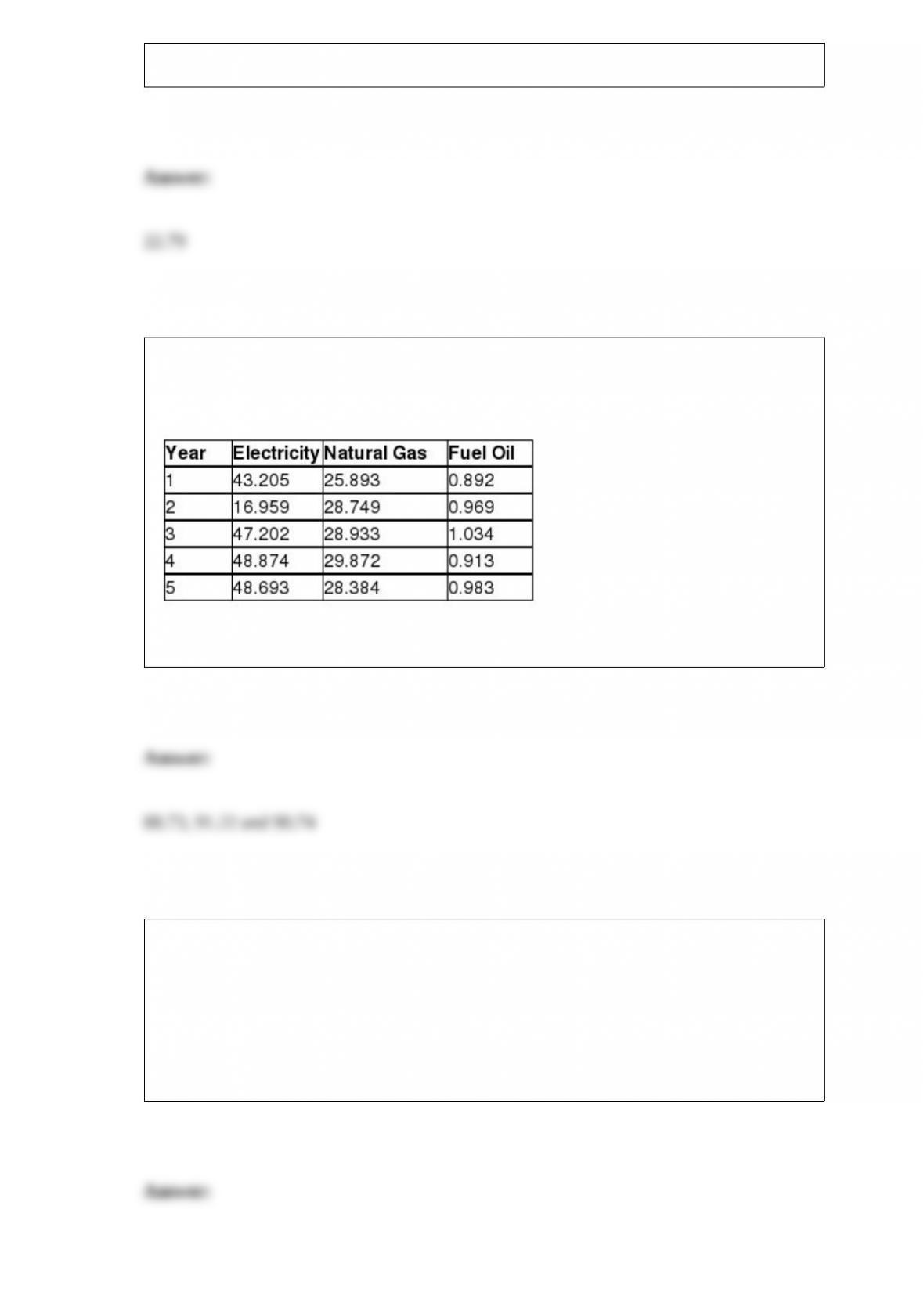
TABLE 16-15
Given below are the average prices for three types of energy products for five
consecutive years.
Referring to Table 16-15, what are the simple price indices for electricity, natural gas
and fuel oil, respectively, in year 1 using year 5 as the base year?
TABLE 5-5
From an inventory of 48 new cars being shipped to local dealerships, corporate reports
indicate that 12 have defective radios installed.
Referring to Table 5-5, what is the probability out of the 8 new cars it just received that,
when each is tested, no more than half of the cars have defective radios?

Referring to Table 14-10, to test the signiticance of the multiple
regression model, what are the degrees of freedom?
TABLE 14-10
You worked as an intern at We Always Win Car Insurance Company
last summer. You notice that individual car insurance premiums
depend very much on the age of the individual and the number of
traffic tickets received by the individual. You performed a regression
analysis in EXCEL and obtained the following partial information:
TABLE 13-5
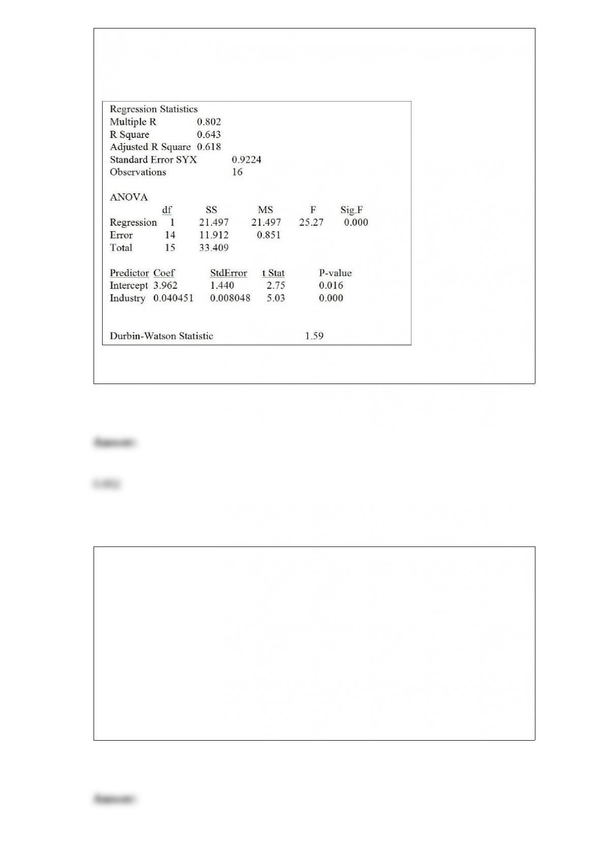
The managing partner of an advertising agency believes that his company’s sales are
related to the industry sales. He uses Microsoft Excel to analyze the last 4 years of
quarterly data (i.e., n = 16) with the following results:
Referring to Table 13-5, the correlation coefficient is ________.
TABLE 6-6
According to Investment Digest, the arithmetic mean of the annual return for common
stocks over an 85-year period was 9.5%, but the value of the variance was not
mentioned. Also 25% of the annual returns were below 8%, while 65% of the annual
returns were between 8% and 11.5%. The article claimed that the distribution of annual
return for common stocks was bell-shaped and approximately symmetric. Assume that
this distribution is normal with the mean given above. Answer the following questions
without the help of a calculator, statistical software or statistical table.
Referring to Table 6-6, find the probability that the annual return of a random year will
be between 7.5% and 11%.