Unlock document.
This document is partially blurred.
Unlock all pages and 1 million more documents.
Get Access
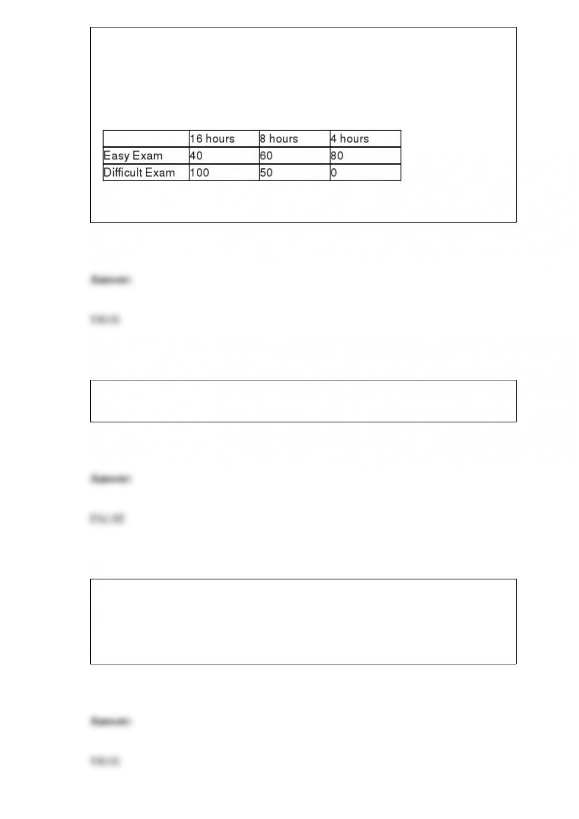
True or False: TABLE 19-6
A student wanted to find out the optimal strategy to study for a Business Statistics
exam. He constructed the following payoff table based on the mean amount of time he
needed to study every week for the course and the degree of difficulty of the exam.
From the information that he gathered from students who had taken the course, he
concluded that there was a 40% probability that the exam would be easy.
Referring to Table 19-6, the optimal strategy using the coefficient of variation criterion
is to study 8 hours per week on average for the exam.
True or False: As a general rule, one can use the normal distribution to approximate a
binomial distribution whenever the sample size is at least 15.
True or False: At a meeting of information systems officers for regional offices of a
national company, a survey was taken to determine the number of employees the
officers supervise in the operation of their departments, where X is the number of
employees overseen by each information systems officer. A stem-and-leaf display can
be used to present this information.
True or False: In a set of numerical data, the value for Q3 can never be smaller than the
value for Q1.
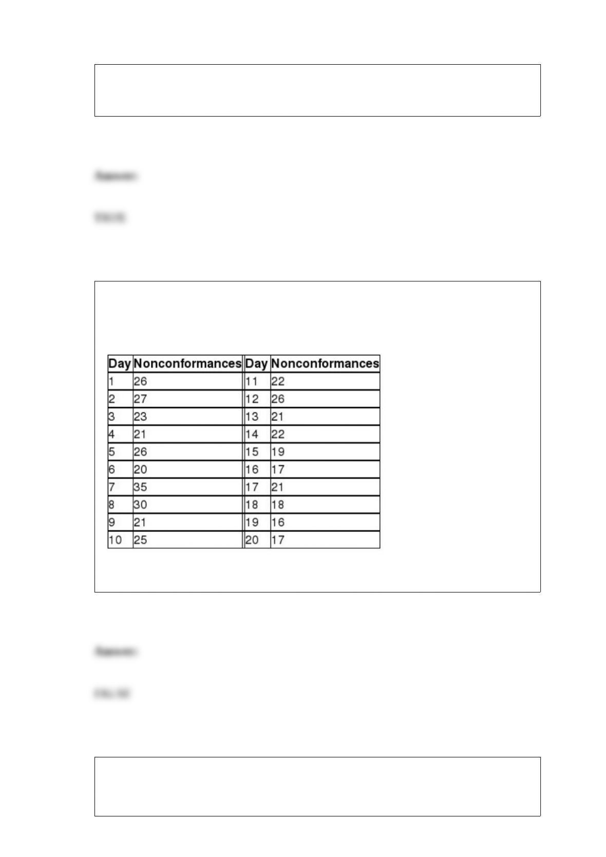
True or False: TABLE 18-10
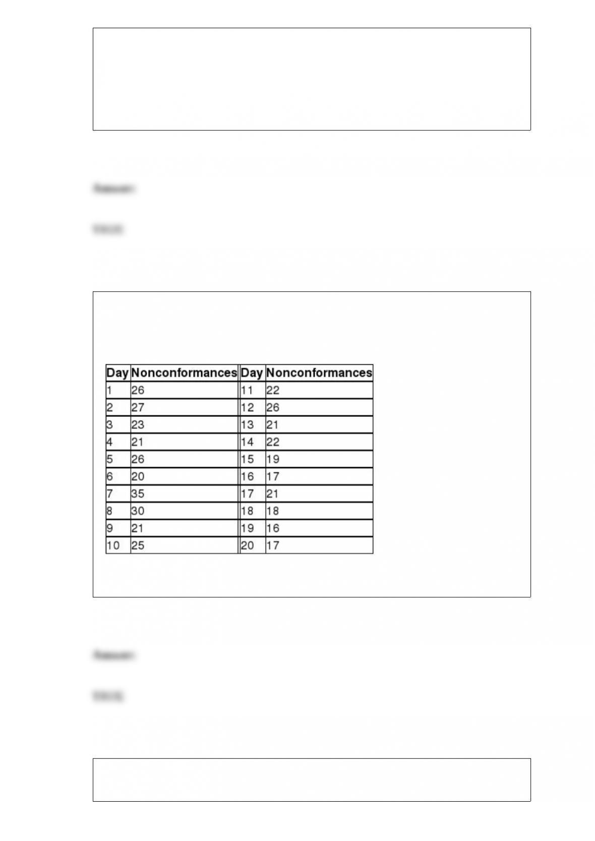
Below is the number of defective items from a production line over twenty consecutive
morning shifts.
Referring to Table 18-10, based on the c chart, no opportunity appears to be present to
render an improvement in the process.
True or False: TABLE 17-8
The superintendent of a school district wanted to predict the percentage of students
passing a sixth-grade proficiency test. She obtained the data on percentage of students
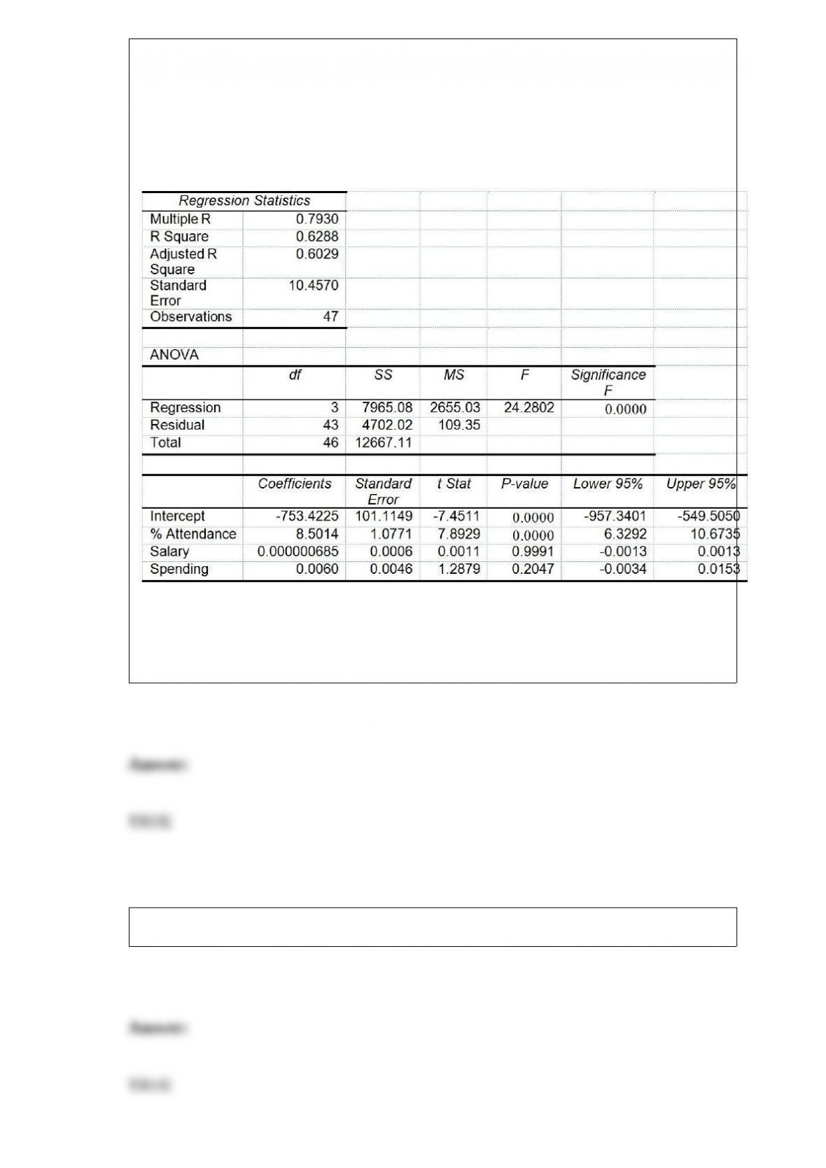
passing the proficiency test (% Passing), daily mean of the percentage of students
attending class (% Attendance), mean teacher salary in dollars (Salaries), and
instructional spending per pupil in dollars (Spending) of 47 schools in the state.
Following is the multiple regression output with Y = % Passing as the dependent
variable, X1 = % Attendance, X2 = Salaries and X3 = Spending:
Referring to Table 17-8, you can conclude that the mean teacher salary individually has
no impact on the mean percentage of students passing the proficiency test, taking into
account the effect of all the other independent variables, at a 1% level of significance
based solely on the 95% confidence interval estimate for β2.
True or False: The control limits are based on the standard deviation of the process.
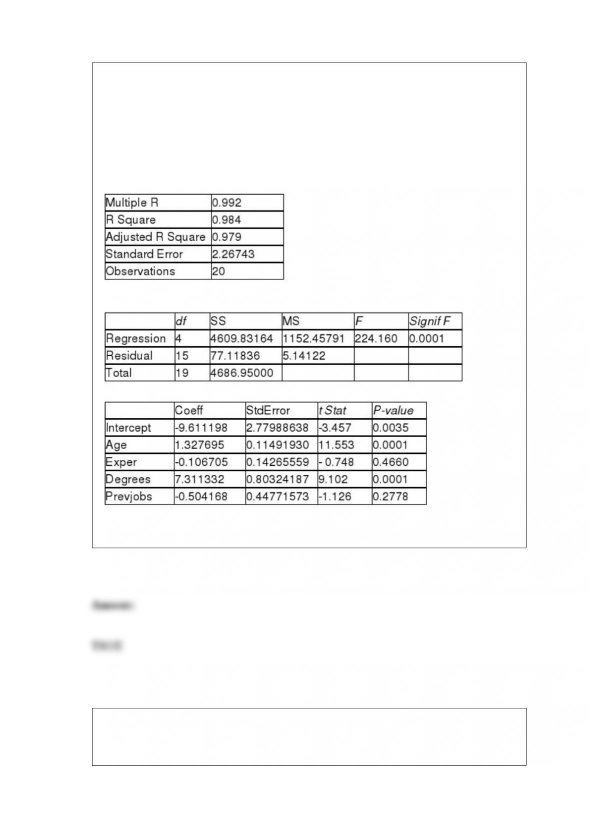
True or False: TABLE 17-3
A financial analyst wanted to examine the relationship between salary (in $1,000) and 4
variables: age (X1 = Age), experience in the field (X2 = Exper), number of degrees (X3 =
Degrees), and number of previous jobs in the field (X4 = Prevjobs). He took a sample of
20 employees and obtained the following Microsoft Excel output:
SUMMARY OUTPUT
Regression Statistics
ANOVA
Referring to Table 17-3, the F test for the significance of the entire regression
performed at a level of significance of 0.01 leads to a rejection of the null hypothesis.
True or False: The expected return of the sum of two investments will be equal to the
sum of the expected returns of the two investments plus twice the covariance between
the investments.

True or False: Holding the width of a confidence interval fixed, increasing the level of
confidence can be achieved with a lower sample size.
TABLE 8-4
The actual voltages of power packs labeled as 12 volts are as follows: 11.77, 11.90,
11.64, 11.84, 12.13, 11.99, and 11.77.
True or False: Referring to Table 8-4, it is possible that the 99% confidence interval
calculated from the data will not contain the mean voltage for the sample.
TABLE 14-15
The superintendent of a school district wanted to predict the
percentage of students passing a sixth-grade proficiency test. She
obtained the data on percentage of students passing the proficiency
test (% Passing), mean teacher salary in thousands of dollars
(Salaries), and instructional spending per pupil in thousands of dollars
(Spending) of 47 schools in the state.
Following is the multiple regression output with Y = % Passing as the
dependent variable, X1 = Salaries and X2 = Spending:

True or False: Referring to Table 14-15, the null hypothesis H0 : β1 =
β2 = 0 implies that percentage of students passing the proficiency
test is not related to one of the explanatory variables.
TABLE 12-3
The director of transportation of a large company is interested in the usage of her van
pool. She considers her routes to be divided into local and non-local. She is particularly
interested in learning if there is a difference in the proportion of males and females who
use the local routes. She takes a sample of a day's riders and finds the following:
She will use this information to perform a chi-square hypothesis test using a level of
significance of 0.05.
True or False: Referring to Table 12-3, the decision made suggests that there is a
difference between the proportion of males and females who ride local versus non-local
routes.
True or False: TABLE 18-10
Below is the number of defective items from a production line over twenty consecutive
morning shifts.
Referring to Table 18-10, based on the c chart, it appears that the process is out of
control.
TABLE 9-6

The quality control engineer for a furniture manufacturer is interested in the mean
amount of force necessary to produce cracks in stressed oak furniture. She performs a
two-tail test of the null hypothesis that the mean for the stressed oak furniture is 650.
The calculated value of the Z test statistic is a positive number that leads to a p-value of
0.080 for the test.
True or False: Referring to Table 9-6, suppose the engineer had decided that the
alternative hypothesis to test was that the mean was less than 650. Then if the test is
performed with a level of significance of 0.05, the null hypothesis would be rejected.
Which of the 4 methods of data collection is involved when a person counts the number
of cars passing designated locations on the Los Angeles freeway system?
A) published sources
B) experimentation
C) surveying
D) observation
TABLE 17-2
One of the most common questions of prospective house buyers pertains to the cost of
heating in dollars (Y). To provide its customers with information on that matter, a large
real estate firm used the following 4 variables to predict heating costs: the daily
minimum outside temperature in degrees of Fahrenheit (X1), the amount of insulation in
inches (X2), the number of windows in the house (X3), and the age of the furnace in
years (X4). Given below are the EXCEL outputs of two regression models.
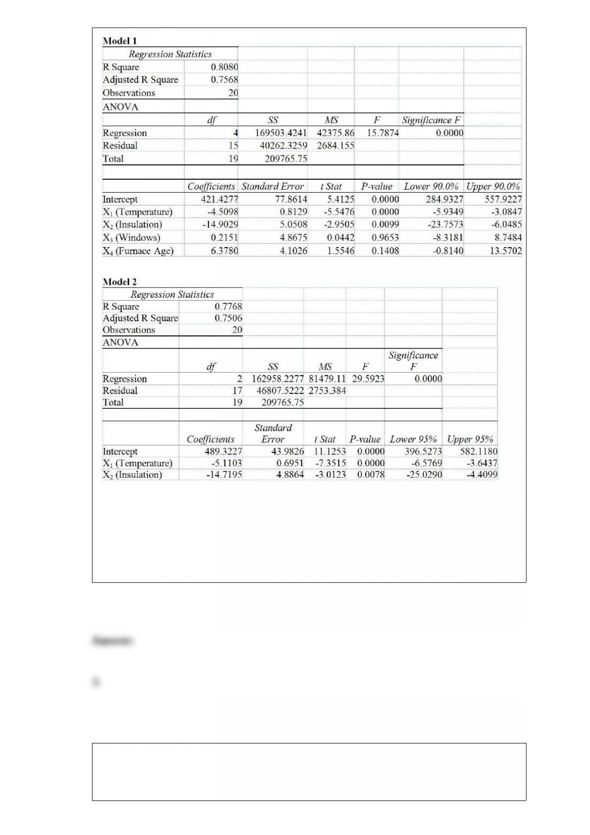
Referring to Table 17-2, what are the degrees of freedom of the partial F test for
H0 : β3 = β4 = 0 vs. H1 : At least one βj ≠0, j = 3, 4?
A) 2 numerator degrees of freedom and 15 denominator degrees of freedom
B) 15 numerator degrees of freedom and 2 denominator degrees of freedom
C) 2 numerator degrees of freedom and 17 denominator degrees of freedom
D) 17 numerator degrees of freedom and 2 denominator degrees of freedom
Data on the amount of time spent studying and the exam score of 150 students at a high
school were collected. You want to know if a student's exam score is linearly related to
the amount of time spent on studying. Which of the following would you compute?
A) Arithmetic mean
B) Median
C) Coefficient of variation
D) Coefficient of correlation
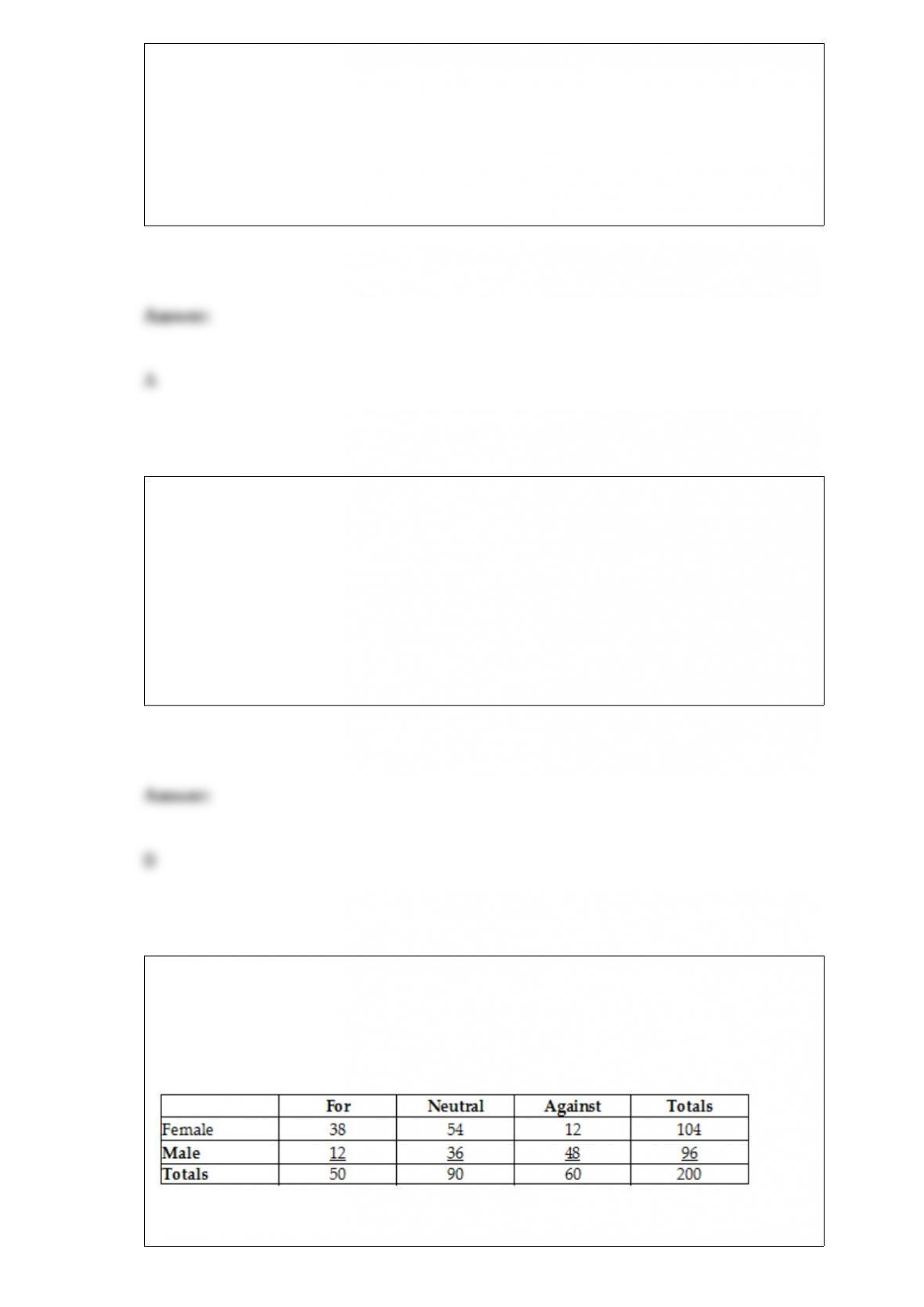
TABLE 17-1
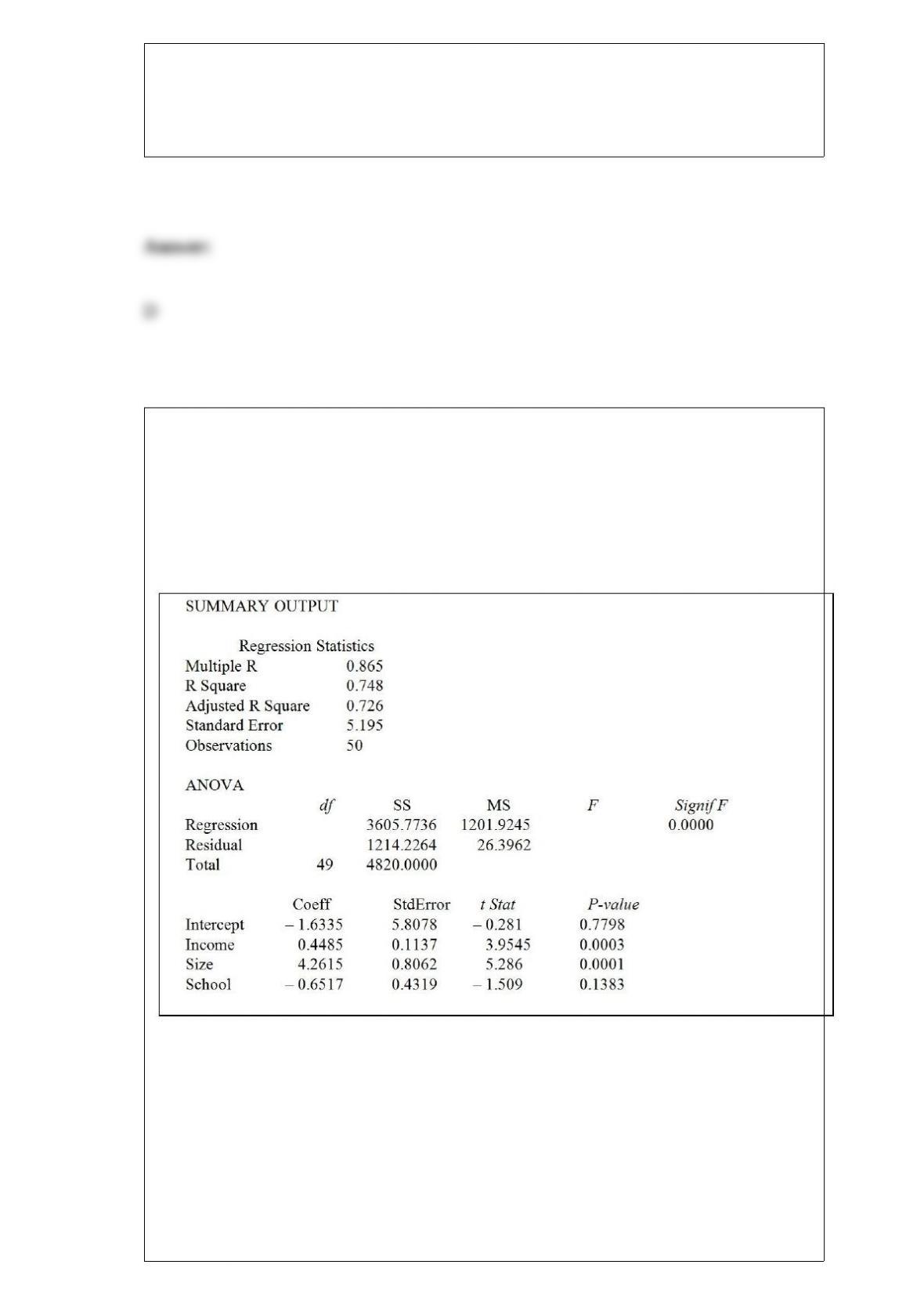
A real estate builder wishes to determine how house size (House) is influenced by
family income (Income), family size (Size), and education of the head of household
(School). House size is measured in hundreds of square feet, income is measured in
thousands of dollars, and education is in years. The builder randomly selected 50
families and ran the multiple regression. Microsoft Excel output is provided below:
Referring to Table 17-1, at the 0.01 level of significance, what conclusion should the
builder draw regarding the inclusion of School in the regression model?
A) School is significant in explaining house size and should be included in the model
because its p-value is less than 0.01.
B) School is significant in explaining house size and should be included in the model
because its p-value is more than 0.01.
C) School is not significant in explaining house size and should not be included in the
model because its p-value is less than 0.01.
D) School is not significant in explaining house size and should not be included in the
model because its p-value is more than 0.01.
In a right-skewed distribution,
A) the median equals the arithmetic mean.
B) the median is less than the arithmetic mean.
C) the median is greater than the arithmetic mean.
D) None of the above.
TABLE 16-3
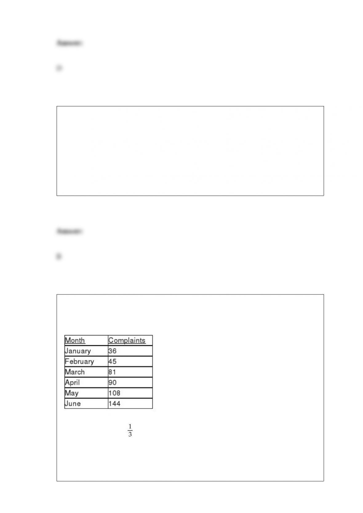
The following table contains the number of complaints received in a department store
for the first 6 months of last year.
Referring to Table 16-3, if this series is smoothed using exponential smoothing with a
smoothing constant of , how many values would it have?
A) 3
B) 4
C) 5
D) 6

A physician and president of a Tampa Health Maintenance Organization (HMO) are
attempting to show the benefits of managed health care to an insurance company. The
physician believes that certain types of doctors are more cost-effective than others. To
investigate this, the president obtained independent random samples of 20 HMO
physicians from each of 4 primary specialties - General Practice (GP), Internal
Medicine (IM), Pediatrics (PED), and Family Physicians (FP) - and recorded the total
charges per member per month for each. A second variable which the president believes
influences total charges per member per month is whether the doctor is a foreign or
USA medical school graduate. To investigate this, the president also collected data on
20 foreign medical school graduates in each of the 4 primary specialty types described
above. Altogether, information on charges for 40 doctors (20 foreign and 20 USA
medical school graduates) was obtained for each of the 4 specialties. The president has
already found out that specialty types and origin of the medical degree do not interact to
affect the charges. He has also found out special types do have an impact on average
charges. Which of the following tests will be the most appropriate to find out which
primary specialty has the highest charges?
A) Tukey-Kramer multiple comparisons procedure for one-way ANOVA
B) Tukey multiple comparisons procedure for two-way ANOVA
C) Two-way ANOVA F test for primary specialty effect
D) Two-way ANOVA F test for origin of the medical degree effect
TABLE 3-11
Given below are the closing prices for the Dow Jones Industrial Average (DJIA) and the
Standard & Poor's (S&P) 500 Index over 10 weeks.
Referring to Table 3-11, you will expect an increase in the DJIA to be associated with
A) an increase in the S&P 500 index.
B) a decrease in the S&P 500 index.
C) no predictable change in the DJIA.
D) no predictable change in the S&P 500 index.
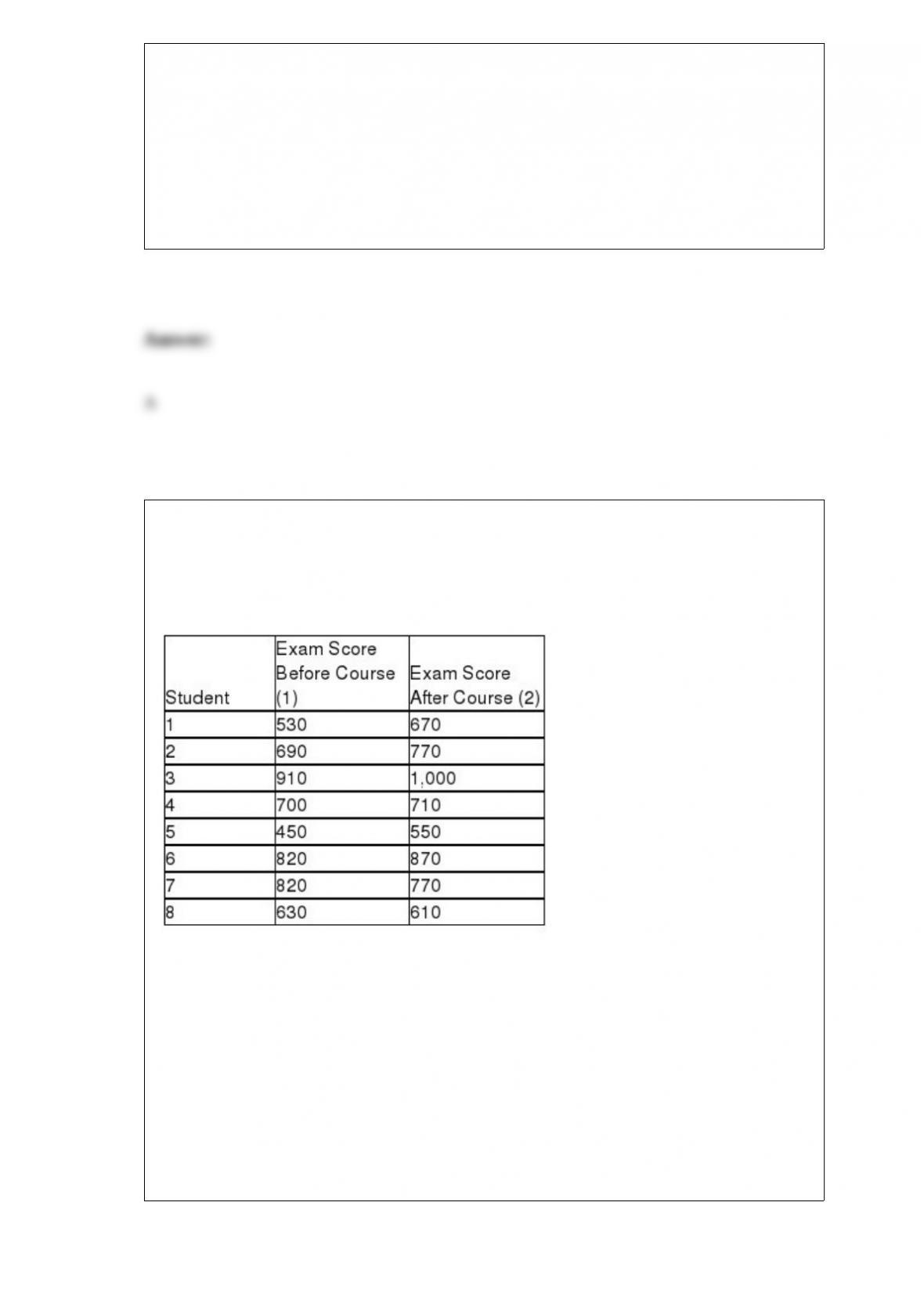
TABLE 10-5
To test the effectiveness of a business school preparation course, 8 students took a
general business test before and after the course. The results are given below.
Referring to Table 10-5, at the 0.05 level of significance, the decision for this
hypothesis test would be
A) reject the null hypothesis.
B) do not reject the null hypothesis.
C) reject the alternative hypothesis.
D) It cannot be determined from the information given.
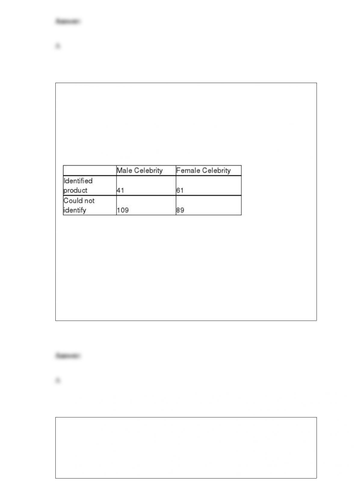
TABLE 12-9
Many companies use well-known celebrities as spokespersons in their TV
advertisements. A study was conducted to determine whether brand awareness of
female TV viewers and the gender of the spokesperson are independent. Each in a
sample of 300 female TV viewers was asked to identify a product advertised by a
celebrity spokesperson. The gender of the spokesperson and whether or not the viewer
could identify the product was recorded. The numbers in each category are given below.
Referring to Table 12-9, at 5% level of significance, the critical value of the test statistic
is
A) 3.8415.
B) 5.9914.
C) 9.4877.
D) 13.2767.
TABLE 10-3
A real estate company is interested in testing whether the mean time that families in
Gotham have been living in their current homes is less than families in Metropolis.
Assume that the two population variances are equal. A random sample of 100 families
from Gotham and a random sample of 150 families in Metropolis yield the following

data on length of residence in current homes.
Gotham: G = 35 months, = 900 Metropolis: M = 50 months, = 1050
Referring to Table 10-3, suppose = 0.01. Which of the following represents the correct
conclusion?
A) There is not enough evidence that the mean amount of time families in Gotham have
been living in their current homes is less than families in Metropolis.
B) There is enough evidence that the mean amount of time families in Gotham have
been living in their current homes is less than families in Metropolis.
C) There is not enough evidence that the mean amount of time families in Gotham have
been living in their current homes is not less than families in Metropolis.
D) There is enough evidence that the mean amount of time families in Gotham have
been living in their current homes is not less than families in Metropolis.
TABLE 13-12
The manager of the purchasing department of a large saving and loan organization
would like to develop a model to predict the amount of time (measured in hours) it
takes to record a loan application. Data are collected from a sample of 30 days, and the
number of applications recorded and completion time in hours is recorded. Below is the
regression output:
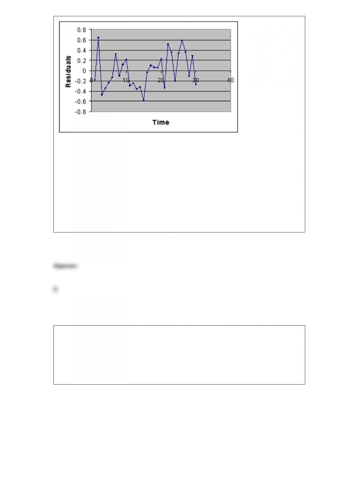
Referring to Table 13-12, the degree(s) of freedom for the t test on whether the number
of loan applications recorded affects the amount of time is (are)
A) 1.
B) 28.
C) 29.
D) 30.
TABLE 12-15
Two new different models of compact SUVs have just arrived at the market. You are
interested in comparing the gas mileage performance of both models to see if they are
the same. A partial computer output for twelve compact SUVs of model 1 and thirteen
of model 2 is given below:
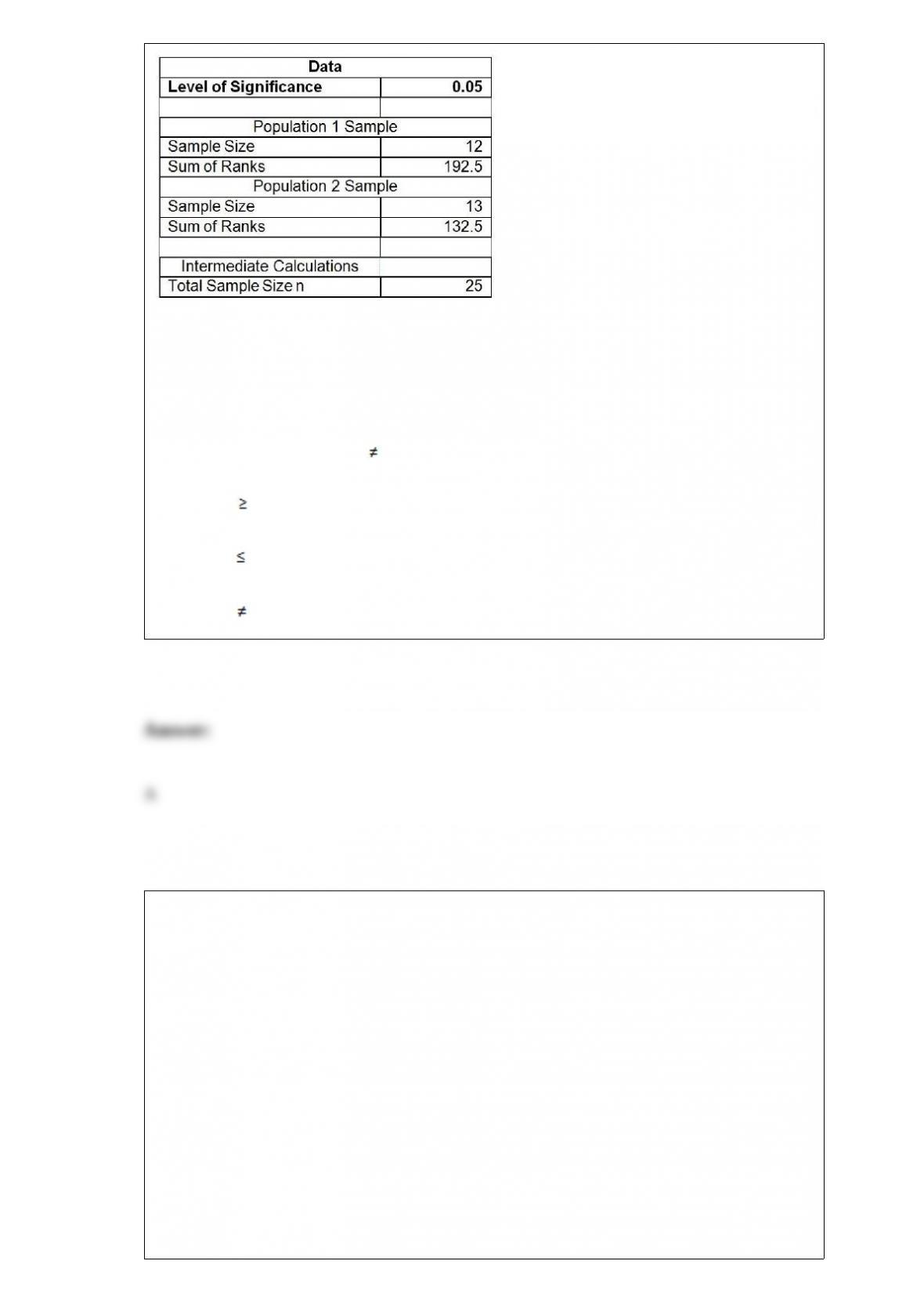
You are told that the gas mileage population distributions for both models are not
normally distributed.
Referring to Table 12-15, what should be the null and alternative hypotheses of the test?
A) H0 : M1 = M2 vs. H1 : M1M2
B) H0 : M1M2 vs. H1 : M1 < M2
C) H0 : M1M2 vs. H1 : M1 > M2
D) H0 : M1M2 vs. H1 : M1 = M2
TABLE 9-3
An appliance manufacturer claims to have developed a compact microwave oven that
consumes a mean of no more than 250 W. From previous studies, it is believed that
power consumption for microwave ovens is normally distributed with a population
standard deviation of 15 W. A consumer group has decided to try to discover if the
claim appears true. They take a sample of 20 microwave ovens and find that they
consume a mean of 257.3 W.
Referring to Table 9-3, the population of interest is
A) the power consumption in the 20 microwave ovens.
B) the power consumption in all such microwave ovens.

C) the mean power consumption in the 20 microwave ovens.
D) the mean power consumption in all such microwave ovens.
TABLE 17-4
You decide to predict gasoline prices in different cities and towns in the United States
for your term project. Your dependent variable is price of gasoline per gallon and your
explanatory variables are per capita income, the number of firms that manufacture
automobile parts in and around the city, the number of new business starts in the last
year, population density of the city, percentage of local taxes on gasoline, and the
number of people using public transportation. You collected data of 32 cities and
obtained a regression sum of squares SSR= 122.8821. Your computed value of standard
error of the estimate is 1.9549.
Referring to Table 17-4, if variables that measure the number of new business starts in
the last year and population density of the city were removed from the multiple
regression model, which of the following would be true?
A) The adjusted r2 will definitely increase.
B) The adjusted r2 cannot increase.
C) The coefficient of multiple determination will not increase.
D) The coefficient of multiple determination will definitely increase.
TABLE 16-7
The executive vice-president of a drug manufacturing firm believes that the demand for
the firm's most popular drug has been evidencing an exponential trend since 1999. She
uses Microsoft Excel to obtain the partial output below. The dependent variable is the
log base 10 of the demand for the drug, while the independent variable is years, where
1999 is coded as 0, 2000 is coded as 1, etc.
SUMMARY OUTPUT
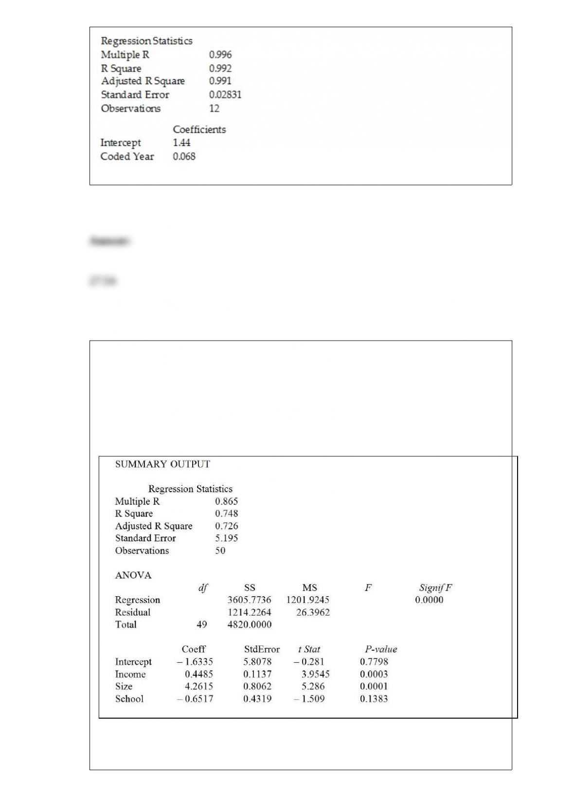
Referring to Table 16-7, the fitted trend value for 1999 is ________.
TABLE 17-1
A real estate builder wishes to determine how house size (House) is influenced by
family income (Income), family size (Size), and education of the head of household
(School). House size is measured in hundreds of square feet, income is measured in
thousands of dollars, and education is in years. The builder randomly selected 50
families and ran the multiple regression. Microsoft Excel output is provided below:
Referring to Table 17-1, at the 0.01 level of significance, what conclusion should the
builder reach regarding the inclusion of Income in the regression model?
A) Income is significant in explaining house size and should be included in the model
because its p-value is less than 0.01.
B) Income is significant in explaining house size and should be included in the model
because its p-value is more than 0.01.
C) Income is not significant in explaining house size and should not be included in the
model because its p-value is less than 0.01.
D) Income is not significant in explaining house size and should not be included in the
model because its p-value is more than 0.01.
Which of the following can be reduced by proper interviewer training?
A) sampling error
B) measurement error
C) Both of the above
D) None of the above
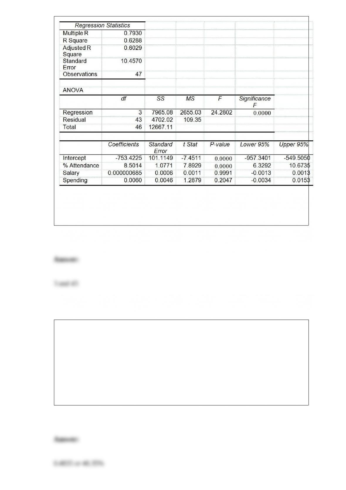
TABLE 2-12
The table below contains the opinions of a sample of 200 people broken down by
gender about the latest congressional plan to eliminate anti-trust exemptions for
professional baseball.
Referring to Table 2-12, of the males in the sample, ________ percent were for the

plan.
In testing for the differences between the means of two related populations, the
________ hypothesis is the hypothesis of "no differences."
TABLE 17-8
The superintendent of a school district wanted to predict the percentage of students
passing a sixth-grade proficiency test. She obtained the data on percentage of students
passing the proficiency test (% Passing), daily mean of the percentage of students
attending class (% Attendance), mean teacher salary in dollars (Salaries), and
instructional spending per pupil in dollars (Spending) of 47 schools in the state.
Following is the multiple regression output with Y = % Passing as the dependent
variable, X1 = % Attendance, X2 = Salaries and X3 = Spending:
Referring to Table 17-8, what are the numerator and denominator degrees of freedom,
respectively, for the test statistic to determine whether there is a significant relationship
between the percentage of students passing the proficiency test and the entire set of
explanatory variables?
TABLE 5-10
An accounting firm in a college town usually recruits employees from two of the
universities in town. This year, there are fifteen graduates from University A and five
from University B and the firm decides to hire six new employees from the two
universities.
Referring to Table 5-10, what is the probability that at least two of the new employees
will be from University B?
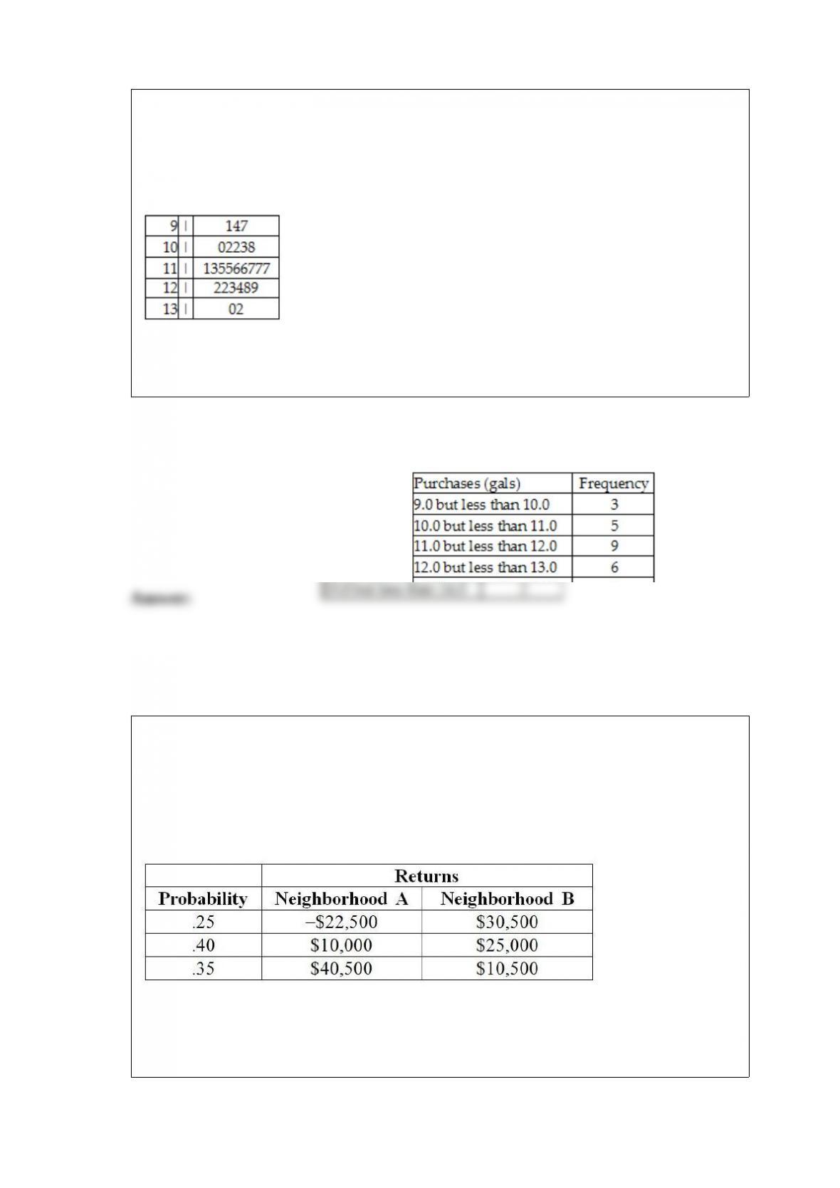
TABLE 2-13
Given below is the stem-and-leaf display representing the amount of detergent used in
gallons (with leaves in 10ths of gallons) in a day by 25 drive-through car wash
operations in Phoenix.
Referring to Table 2-13, construct a frequency distribution for the detergent data, using
"9.0 but less than 10.0 gallons" as the first class.
TABLE 5-7
There are two houses with almost identical characteristics available for investment in
two different neighborhoods with drastically different demographic composition. The
anticipated gain in value when the houses are sold in 10 years has the following
probability distribution:
Referring to Table 5-7, if you can invest 90% of your money on the house in
neighborhood A and the remaining on the house in neighborhood B, what is the
portfolio risk of your investment?

TABLE 6-2
John has two jobs. For daytime work at a jewelry store he is paid $15,000 per month,
plus a commission. His monthly commission is normally distributed with a mean of
$10,000 and a standard deviation of $2,000. At night he works occasionally as a waiter,
for which his monthly income is normally distributed with a mean of $1,000 and a
standard deviation of $300. John's income levels from these two sources are
independent of each other.
Referring to Table 6-2, for a given month, what is the probability that John's income as
a waiter is at least $1,400?


