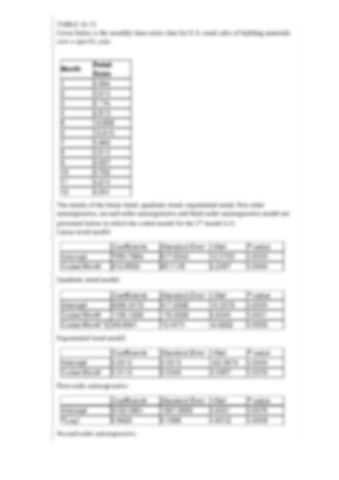
TABLE 16-13
Given below is the monthly time-series data for U.S. retail sales of building materials
over a specific year.
The results of the linear trend, quadratic trend, exponential trend, first-order
autoregressive, second-order autoregressive and third-order autoregressive model are
presented below in which the coded month for the 1st month is 0:
Linear trend model:
Quadratic trend model:
Exponential trend model:
First-order autoregressive:
Second-order autoregressive:
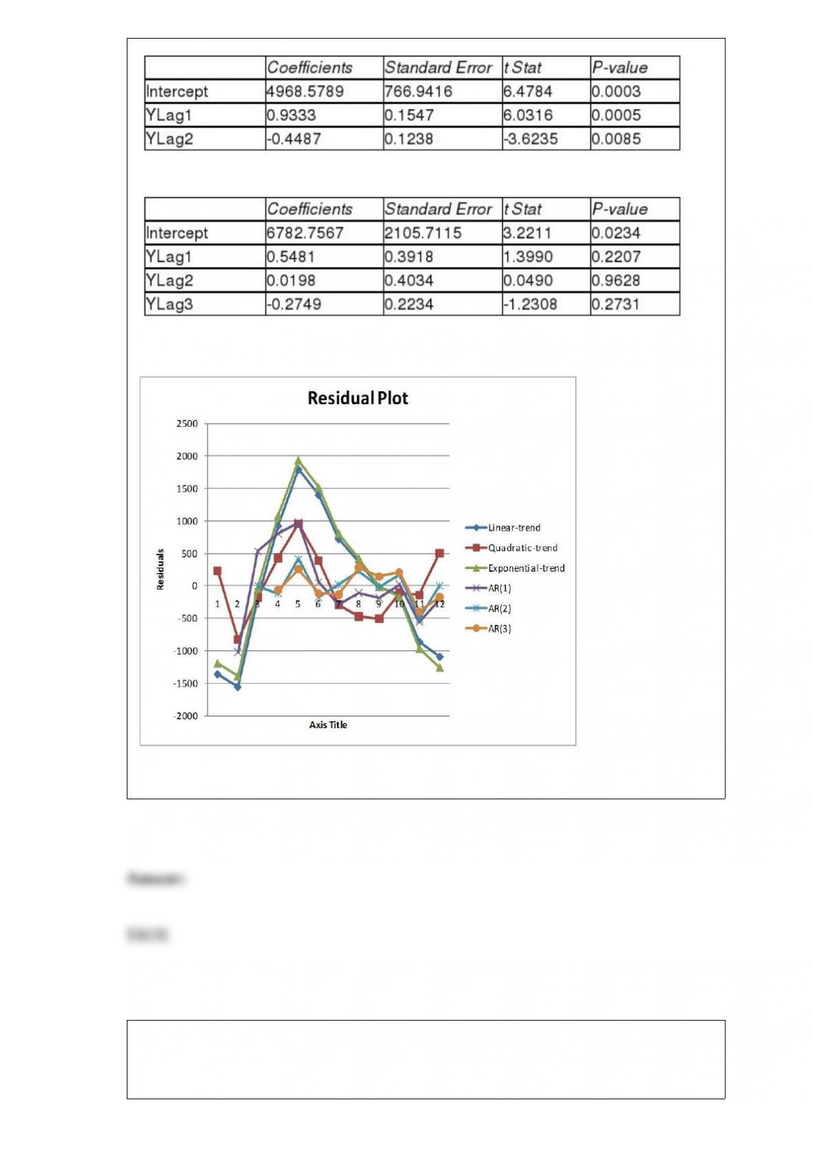
Third-order autoregressive:
Below is the residual plot of the various models:
True or False: Referring to Table 16-13, you can conclude that the second-order
autoregressive model is appropriate at the 5% level of significance.
True or False: A researcher is curious about the effect of sleep on students’ test
performances. He chooses 60 students and gives each two tests: one given after two
hours’ sleep and one after eight hours’ sleep. The test the researcher should use would

be a related samples test.
TABLE 9-9
The president of a university claimed that the entering class this year appeared to be
larger than the entering class from previous years but their mean SAT score is lower
than previous years. He took a sample of 20 of this year’s entering students and found
that their mean SAT score is 1,501 with a standard deviation of 53. The university’s
record indicates that the mean SAT score for entering students from previous years is
1,520. He wants to find out if his claim is supported by the evidence at a 5% level of
significance.
True or False: Referring to Table 9-9, the president can conclude that there is sufficient
evidence to show that the mean SAT score of the entering class this year is lower than
previous years with no more than a 5% probability of incorrectly rejecting the true null
hypothesis.
True or False: The quality (“terrible,” “poor,” “fair”, “acceptable,” “very good,” and
“excellent”) of a day care center is an example of a numerical variable.
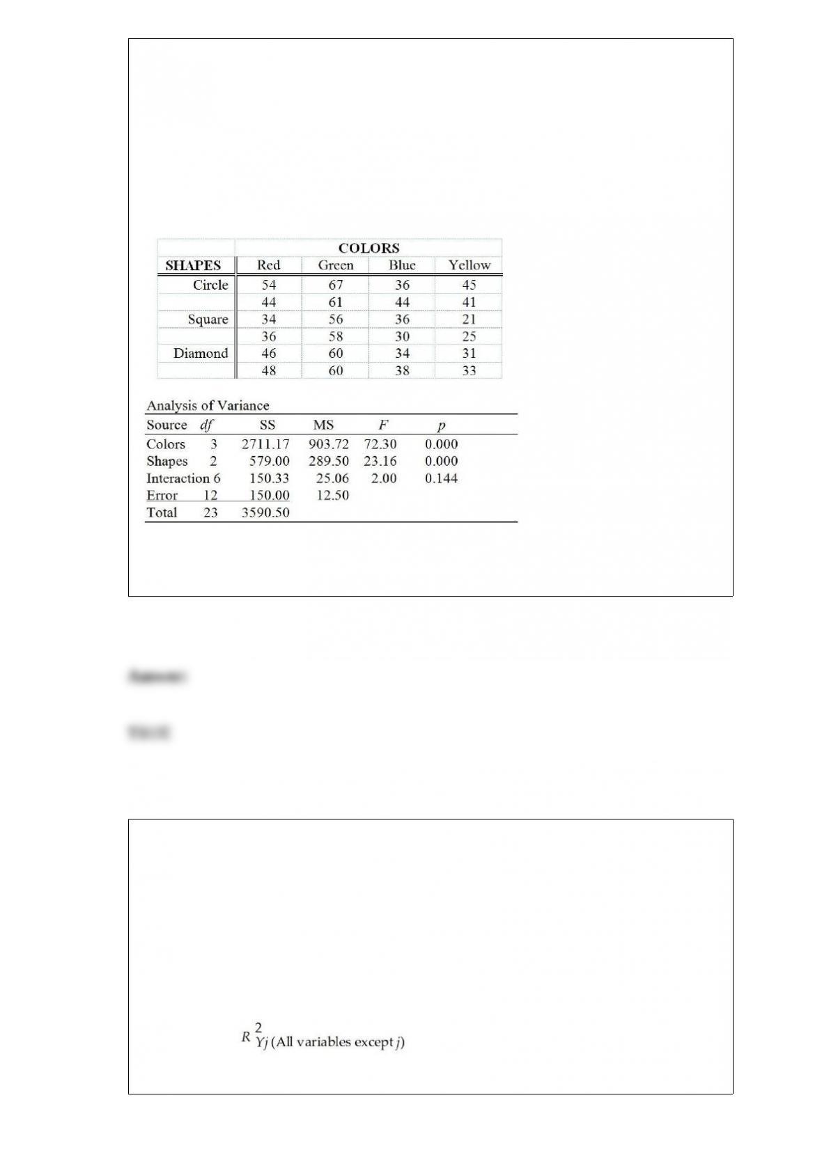
TABLE 11-9
The marketing manager of a company producing a new cereal aimed for children wants
to examine the effect of the color and shape of the box’s logo on the approval rating of
the cereal. He combined 4 colors and 3 shapes to produce a total of 12 designs. Each
logo was presented to 2 different groups (a total of 24 groups) and the approval rating
for each was recorded and is shown below. The manager analyzed these data using the
α = 0.05 level of significance for all inferences.
True or False: Referring to Table 11-9, based on the results of the hypothesis test, it
appears that there is a significant effect associated with the shape of the logo.
TABLE 17-10
Given below are results from the regression analysis where the dependent variable is
the number of weeks a worker is unemployed due to a layoff (Unemploy) and the
independent variables are the age of the worker (Age), the number of years of education
received (Edu), the number of years at the previous job (Job Yr), a dummy variable for
marital status (Married: 1 = married, 0 = otherwise), a dummy variable for head of
household (Head: 1 = yes, 0 = no) and a dummy variable for management position
(Manager: 1 = yes, 0 = no). We shall call this Model 1. The coefficient of partial
determination ( ) of each of the 6 predictors are, respectively,
0.2807, 0.0386, 0.0317, 0.0141, 0.0958, and 0.1201.
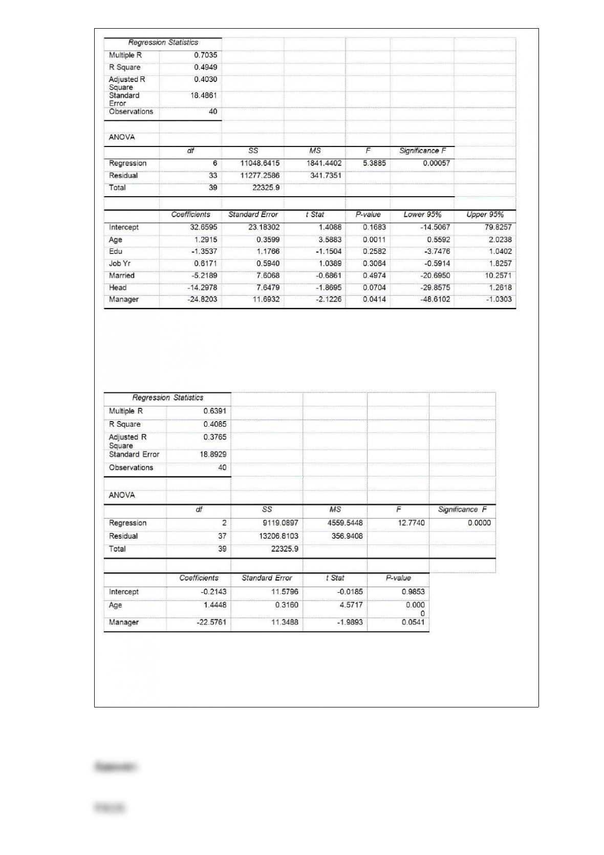
Model 2 is the regression analysis where the dependent variable is Unemploy and the
independent variables are Age and Manager. The results of the regression analysis are
given below:
Referring to Table 17-10, Model 1, the null hypothesis H0 : β1 = β2= β3 = β4 = β5 = β6
= 0 implies that the number of weeks a worker is unemployed due to a layoff is not
related to any of the explanatory variables.
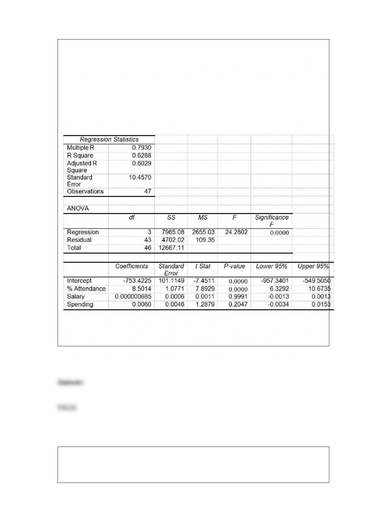
True or False: TABLE 17-8
The superintendent of a school district wanted to predict the percentage of students
passing a sixth-grade proficiency test. She obtained the data on percentage of students
passing the proficiency test (% Passing), daily mean of the percentage of students
attending class (% Attendance), mean teacher salary in dollars (Salaries), and
instructional spending per pupil in dollars (Spending) of 47 schools in the state.
Following is the multiple regression output with Y = % Passing as the dependent
variable, X1 = % Attendance, X2 = Salaries and X3 = Spending:
Referring to Table 17-8, the alternative hypothesis H1 : At least one of βj ≠0 for j =
1, 2, 3 implies that the percentage of students passing the proficiency test is affected by
at least one of the explanatory variables.
True or False: A race car driver tested his car for time from 0 to 60 mph, and for 20 tests
obtained a mean of 4.85 seconds with a standard deviation of 1.47 seconds. A 95%
confidence interval for the 0 to 60 mean time is 4.52 seconds to 5.18 seconds.
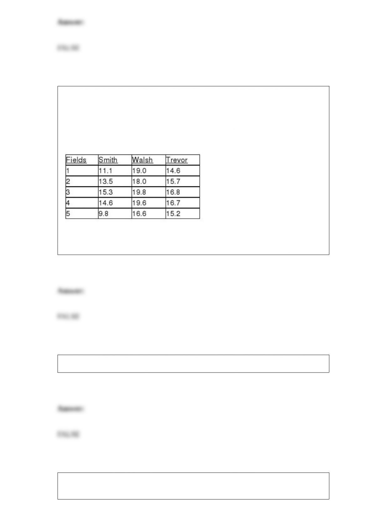
TABLE 11-10
An agronomist wants to compare the crop yield of 3 varieties of chickpea seeds. She
plants all 3 varieties of the seeds on each of 5 different patches of fields. She then
measures the crop yield in bushels per acre. Treating this as a randomized block design,
the results are presented in the table that follows.
True or False: Referring to Table 11-10, the null hypothesis for the F test for the block
effects should be rejected at a 0.01 level of significance.
True or False: Marital status is an example of an ordinal scaled variable.
True or False: TABLE 17-11
A logistic regression model was estimated in order to predict the probability that a
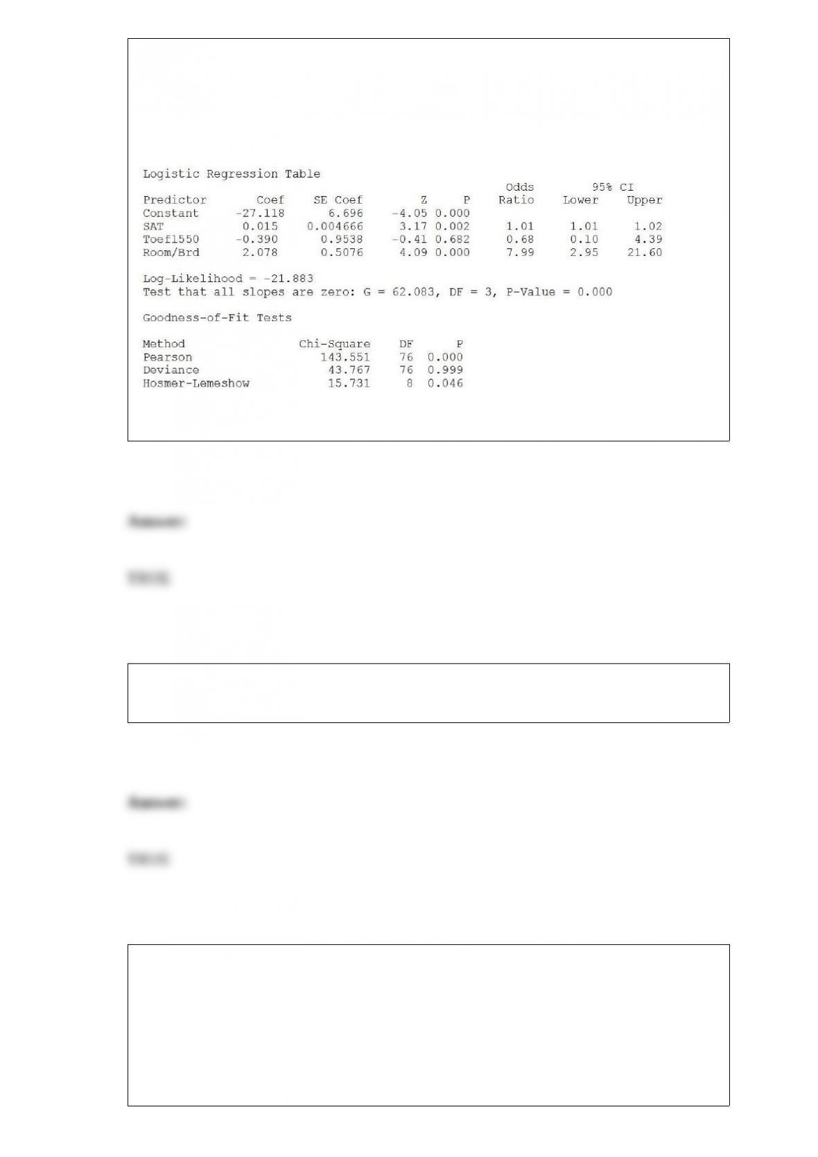
randomly chosen university or college would be a private university using information
on mean total Scholastic Aptitude Test score (SAT) at the university or college, the
room and board expense measured in thousands of dollars (Room/Brd), and whether the
TOEFL criterion is at least 550 (Toefl550 = 1 if yes, 0 otherwise.) The dependent
variable, Y, is school type (Type = 1 if private and 0 otherwise).
Referring to Table 17-11, the null hypothesis that the model is a good-fitting model
cannot be rejected when allowing for a 5% probability of making a type I error.
True or False: One of the advantages of a pie chart is that it clearly shows that the total
of all the categories of the pie adds to 100%.
TABLE 8-8
The president of a university would like to estimate the proportion of the student
population that owns a personal computer. In a sample of 500 students, 417 own a
personal computer.
True or False: Referring to Table 8-8, a 90% confidence interval calculated from the

same data would be narrower than a 99% confidence interval.
True or False: The professor of a business statistics class wanted to find out the mean
amount of time per week her students spent studying for the class. Among the 50
students in her class, 20% were freshmen, 50% were sophomores and 30% were
juniors. She decided to select 2 students randomly from the freshmen, 5 randomly from
the sophomores and 3 randomly from the juniors. This is an example of a systematic
sample.
TABLE 8-11
A poll was conducted by the marketing department of a video game company to
determine the popularity of a new game that was targeted to be launched in three
months. Telephone interviews with 1,500 young adults were conducted which revealed
that 49% said they would purchase the new game. The margin of error was 3
percentage points.
True or False: Referring to Table 8-11, you are 99% confident that the percentage of the
targeted young adults who will purchase the new game is somewhere between 46% and
52%.
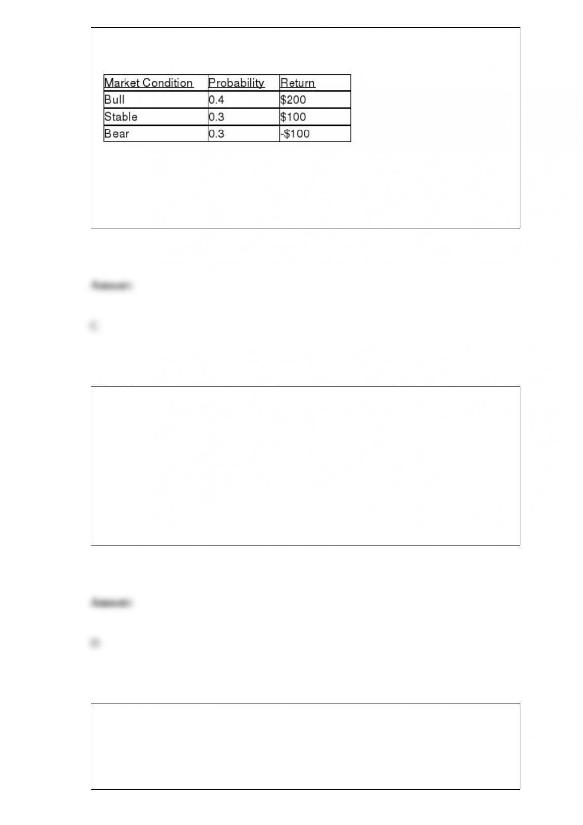
TABLE 19-4
A stock portfolio has the following returns under the market conditions listed below.
Referring to Table 19-4, what is the standard deviation?
A) 4,890
B) 4,840
C) 124.9
D) 69.6
Data on the number of part-time hours students at a public university worked in a week
were collected. Which of the following is the best chart for presenting the information?
A) a pie chart
B) a Pareto chart
C) a percentage table
D) a percentage polygon
The classification of student class designation (freshman, sophomore, junior, senior) is
an example of
A) a categorical variable.
B) a discrete variable.
C) a continuous variable.
D) a table of random numbers.
TABLE 10-3
A real estate company is interested in testing whether the mean time that families in
Gotham have been living in their current homes is less than families in Metropolis.
Assume that the two population variances are equal. A random sample of 100 families
from Gotham and a random sample of 150 families in Metropolis yield the following
data on length of residence in current homes.
Gotham: G = 35 months, = 900 Metropolis: M = 50 months, = 1050
Referring to Table 10-3, suppose = 0.05. Which of the following represents the result
of the relevant hypothesis test?
A) The alternative hypothesis is rejected.
B) The null hypothesis is rejected.
C) The null hypothesis is not rejected.
D) Insufficient information exists on which to make a decision.
Determining the root causes of why defects can occur along with the variables in the
process that cause these defects to occur involves which part of the DMAIC process?
A) Define
B) Measure
C) Analyze
D) Improve
E) Control
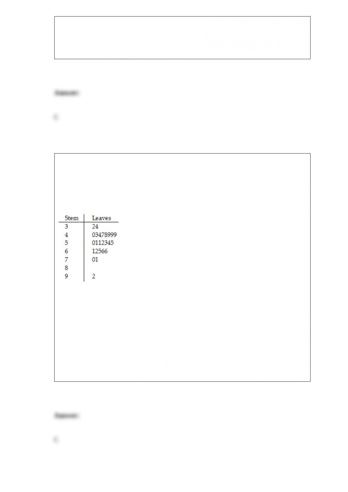
TABLE 2-4
A survey was conducted to determine how people rated the quality of programming
available on television. Respondents were asked to rate the overall quality from 0 (no
quality at all) to 100 (extremely good quality). The stem-and-leaf display of the data is
shown below.
Referring to Table 2-4, what percentage of the respondents rated overall television
quality with a rating of 50 or below?
A) 11
B) 40
C) 44
D) 56
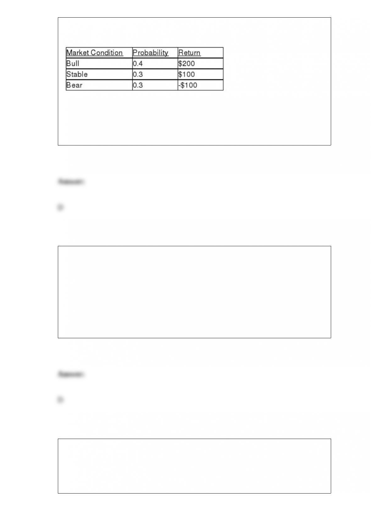
TABLE 19-4
A stock portfolio has the following returns under the market conditions listed below.
Referring to Table 19-4, what is the EMV?
A) $180
B) $130
C) $90
D) $80
Which of the following is most likely a population as opposed to a sample?
A) respondents to a newspaper survey
B) the first 5 students completing an assignment
C) every third person to arrive at the bank
D) registered voters in a county
TABLE 18-3
A quality control analyst for a light bulb manufacturer is concerned that the time it takes
to produce a batch of light bulbs is too erratic. Accordingly, the analyst randomly
surveys 10 production periods each day for 14 days and records the sample mean and
range for each day.
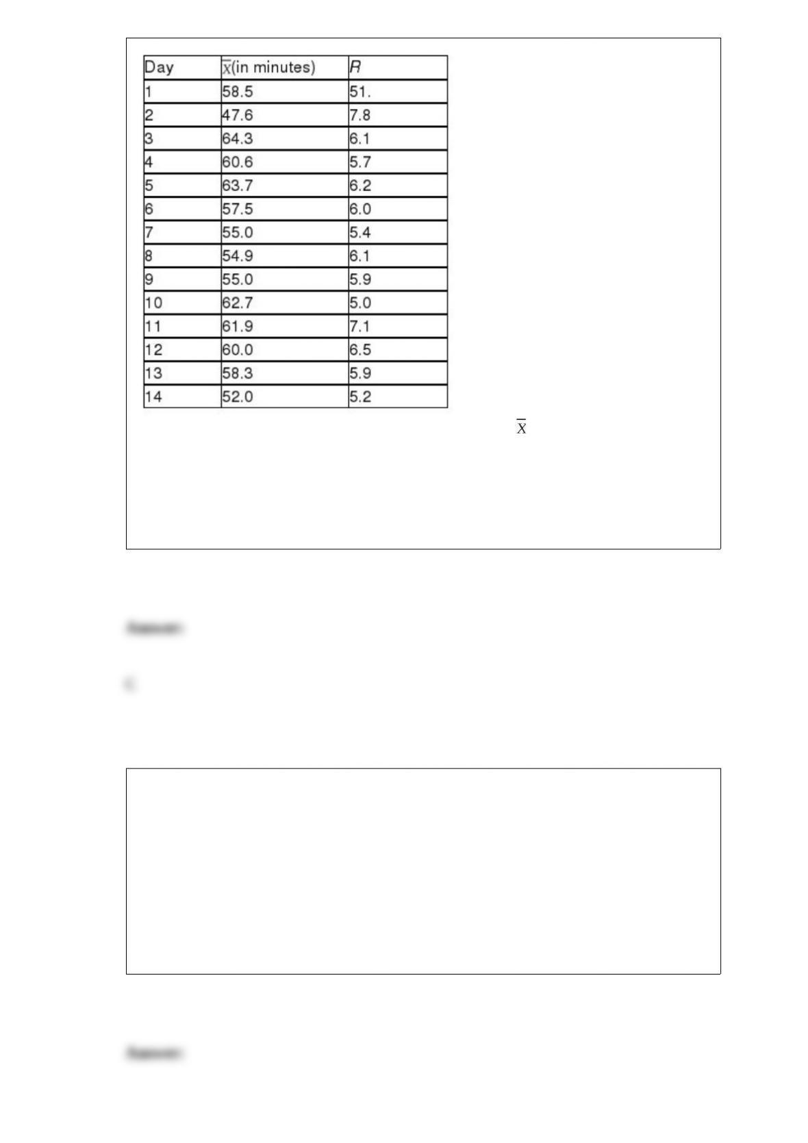
Referring to Table 18-3, suppose the analyst constructs an chart to see if the
production process is in-control. What is the center line for this chart?
A) 64.3
B) 59.5
C) 58.0
D) 57.1
The slope (b1) represents
A) predicted value of Y when X = 0.
B) the estimated average change in Y per unit change in X.
C) the predicted value of Y.
D) variation around the line of regression.

Referring to Table 14-13, the tted model for predicting demand in
Los Angeles is ________.
TABLE 14-13
An econometrician is interested in evaluating the relationship of
demand for building materials to mortgage rates in Los Angeles and
San Francisco. He believes that the appropriate model is
Y = 10 + 5X1 + 8X2
where X1 = mortgage rate in %
X2 = 1 if SF, 0 if LA
Y = demand in $100 per capita
A) 10 + 5X1
B) 10 + 13X1
C) 15 + 8X2
D) 18 + 5X2
TABLE 13-9
It is believed that, the average numbers of hours spent studying per day (HOURS)
during undergraduate education should have a positive linear relationship with the
starting salary (SALARY, measured in thousands of dollars per month) after graduation.
Given below is the Excel output for predicting starting salary (Y) using number of hours
spent studying per day (X) for a sample of 51 students. NOTE: Only partial output is
shown.
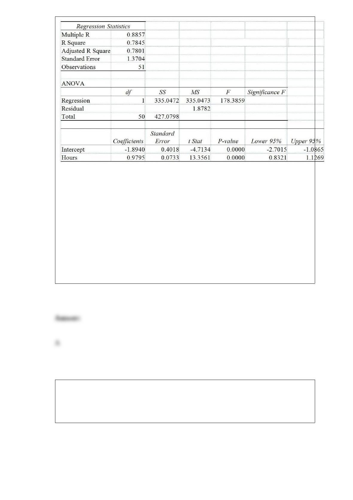
Note: 2.051E – 05 = 2.051 ∗ 10-05 and 5.944E – 18 = 5.944 ∗ 10-18.
Referring to Table 13-9, the degrees of freedom for the F test on whether HOURS
affects SALARY are
A) 1, 49.
B) 1, 50.
C) 49, 1.
D) 50, 1.
TABLE 18-2
A political pollster randomly selects a sample of 100 voters each day for 8 successive
days and asks how many will vote for the incumbent. The pollster wishes to construct a
p chart to see if the percentage favoring the incumbent candidate is too erratic.
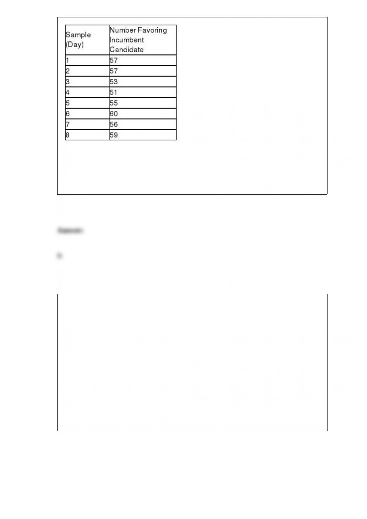
Referring to Table 18-2, what is the numerical value of the center line for the p chart?
A) 0.53
B) 0.56
C) 0.63
D) 0.66
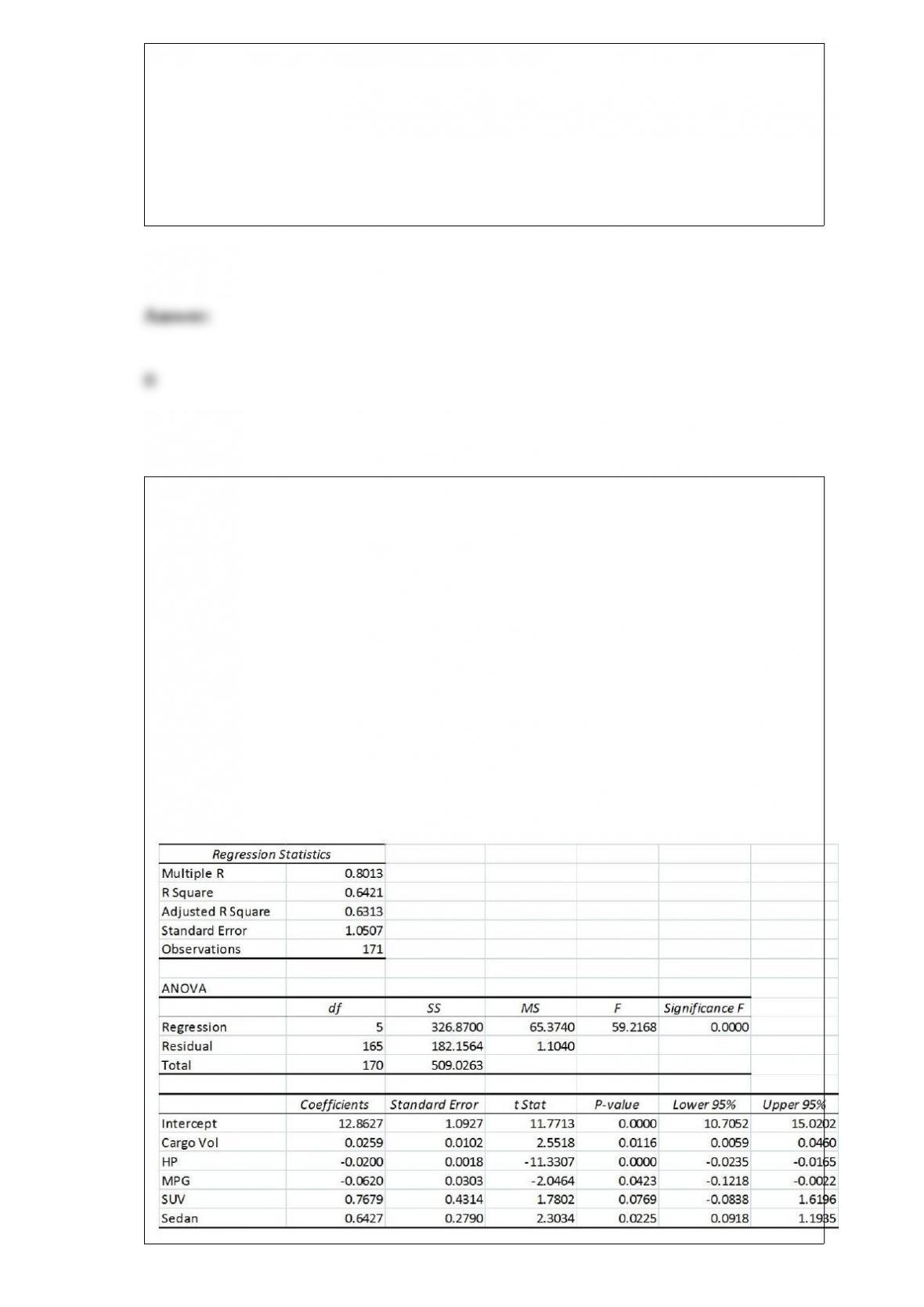
TABLE 17-9
What are the factors that determine the acceleration time (in sec.) from 0 to 60 miles per
hour of a car? Data on the following variables for 171 different vehicle models were
collected:
Accel Time: Acceleration time in sec.
Cargo Vol: Cargo volume in cu. ft.
HP: Horsepower
MPG: Miles per gallon
SUV: 1 if the vehicle model is an SUV with Coupe as the base when SUV and Sedan
are both 0
Sedan: 1 if the vehicle model is a sedan with Coupe as the base when SUV and Sedan
are both 0
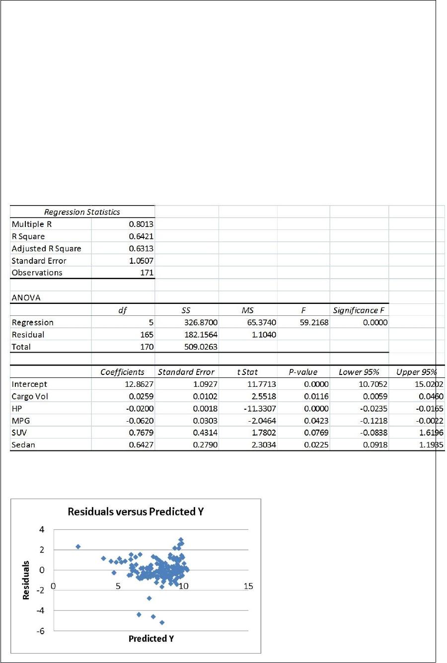
The regression results using acceleration time as the dependent variable and the
remaining variables as the independent variables are presented below.
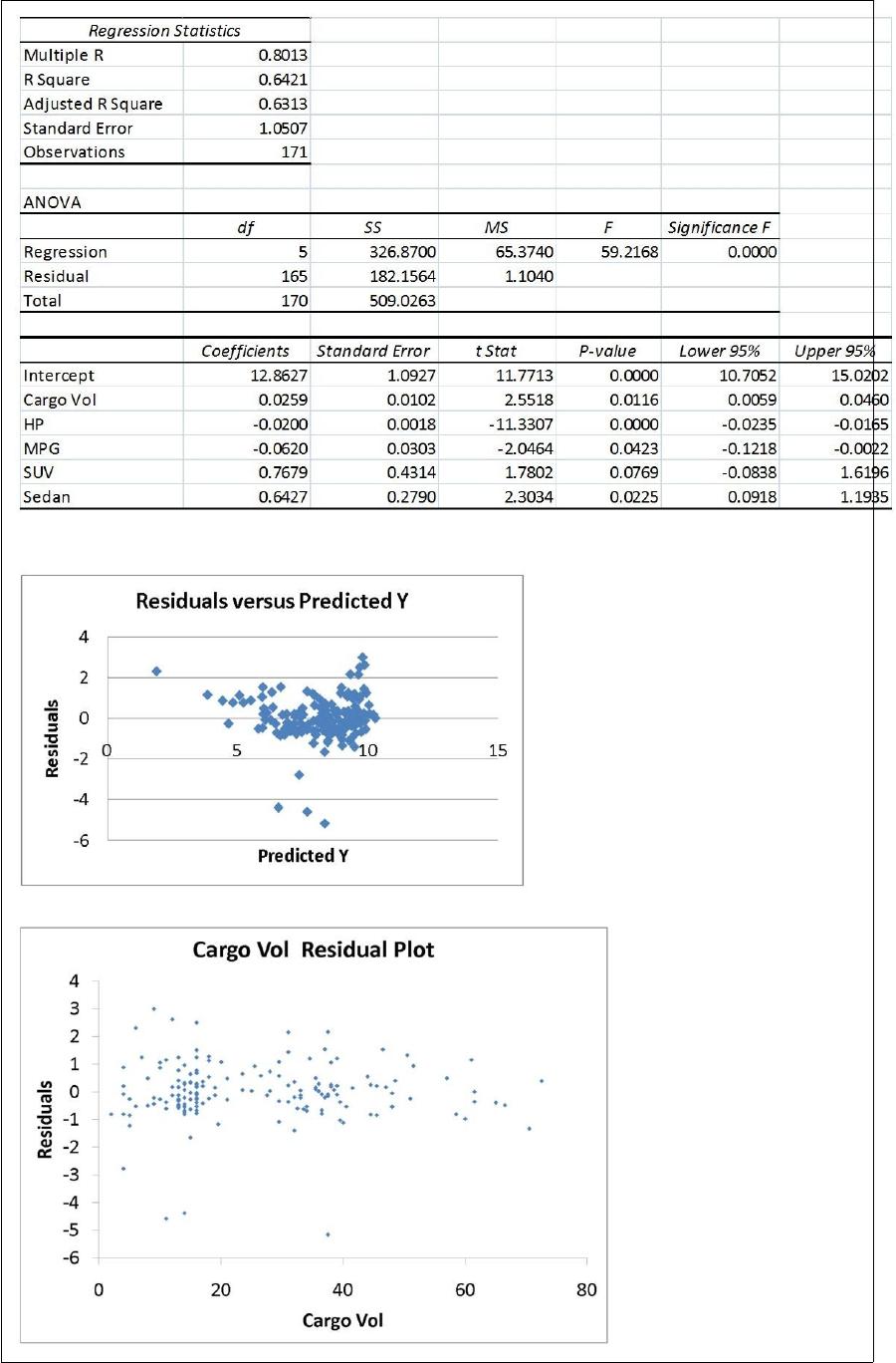
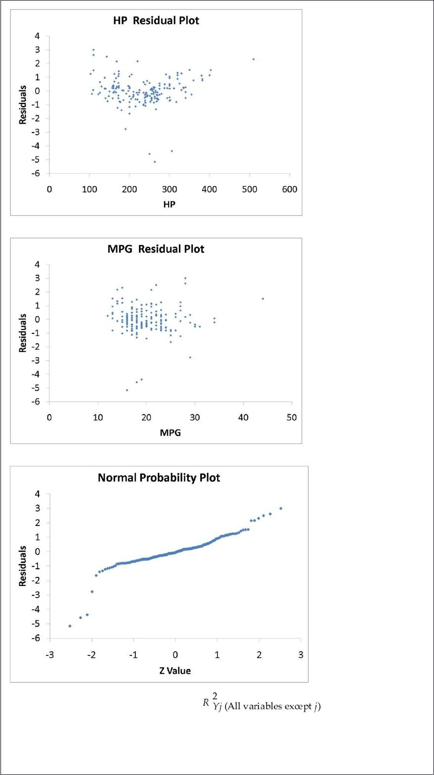
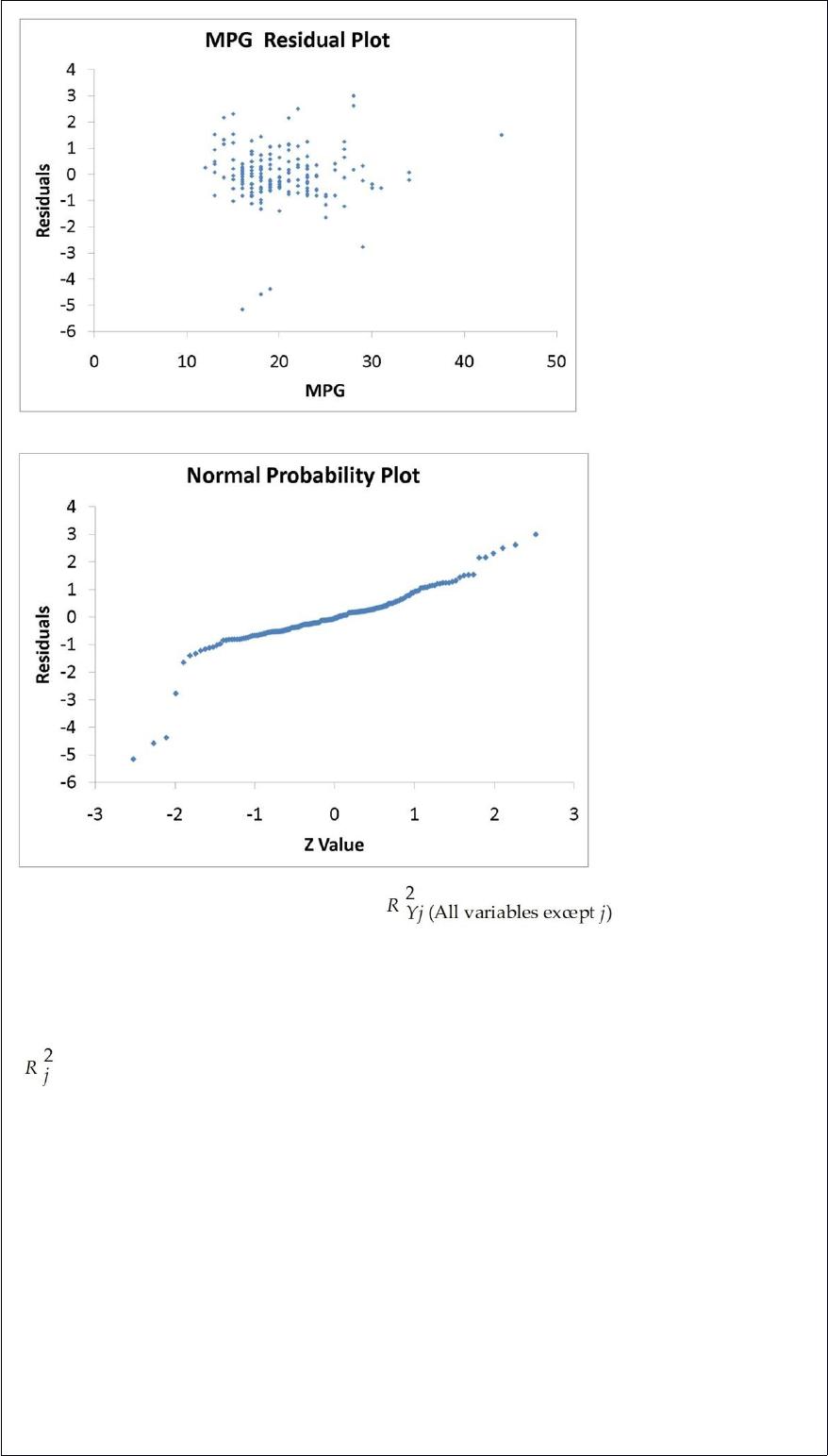
The various residual plots are as shown below.
The coefficient of partial determination ( ) of each of the 5
predictors are, respectively, 0.0380, 0.4376, 0.0248, 0.0188, and 0.0312.
The coefficient of multiple determination for the regression model using each of the 5
variables Xj as the dependent variable and all other X variables as independent variables

( ) are, respectively, 0.7461, 0.5676, 0.6764, 0.8582, 0.6632.
Referring to Table 17-9, what is the correct interpretation for the estimated coefficient
for Sedan?
A) The mean 0 to 60 miles per hour acceleration time of a sedan is estimated to be
0.6427 seconds higher than that of a coupe after considering the effect of all the other
independent variables in the model.
B) The mean 0 to 60 miles per hour acceleration time of a sedan is estimated to be
0.6427 seconds higher than that of an SUV after considering the effect of all the other
independent variables in the model.
C) The mean 0 to 60 miles per hour acceleration time of a sedan is estimated to be
0.6427 seconds lower than that of a coupe after considering the effect of all the other
independent variables in the model.
D) The mean 0 to 60 miles per hour acceleration time of a sedan is estimated to be
0.6427 seconds lower than that of an SUV after considering the effect of all the other
independent variables in the model.
In testing a hypothesis using the X2 test, the theoretical frequencies are based on the
A) null hypothesis.
B) alternative hypothesis.
C) normal distribution.
D) None of the above.
The least squares method minimizes which of the following?
A) SSR
B) SSE
C) SST
D) All of the above.
TABLE 17-9
What are the factors that determine the acceleration time (in sec.) from 0 to 60 miles per
hour of a car? Data on the following variables for 171 different vehicle models were
collected:
Accel Time: Acceleration time in sec.
Cargo Vol: Cargo volume in cu. ft.
HP: Horsepower
MPG: Miles per gallon
SUV: 1 if the vehicle model is an SUV with Coupe as the base when SUV and Sedan
are both 0
Sedan: 1 if the vehicle model is a sedan with Coupe as the base when SUV and Sedan
are both 0
The regression results using acceleration time as the dependent variable and the
remaining variables as the independent variables are presented below.
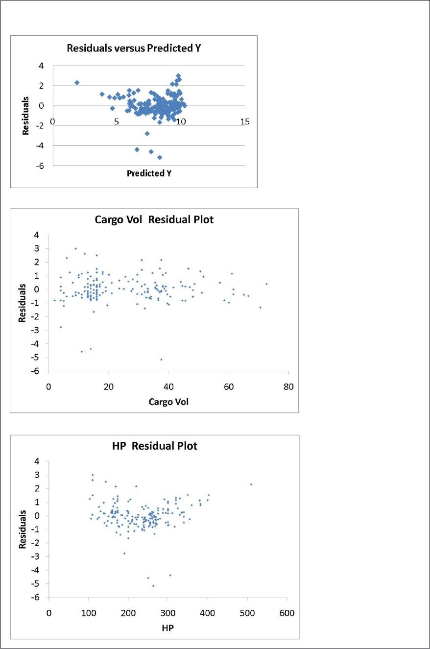
The various residual plots are as shown below.
The coefficient of partial determination ( ) of each of the 5
predictors are, respectively, 0.0380, 0.4376, 0.0248, 0.0188, and 0.0312.
The coefficient of multiple determination for the regression model using each of the 5
variables Xj as the dependent variable and all other X variables as independent variables
( ) are, respectively, 0.7461, 0.5676, 0.6764, 0.8582, 0.6632.
Referring to Table 17-9, what is the correct interpretation for the estimated coefficient
for SUV?
A) The mean 0 to 60 miles per hour acceleration time of an SUV is estimated to be
0.7679 seconds higher than that of a coupe after considering the effect of all the other
independent variables in the model.
B) The mean 0 to 60 miles per hour acceleration time of an SUV is estimated to be
0.7679 seconds higher than that of a sedan after considering the effect of all the other
independent variables in the model.
C) The mean 0 to 60 miles per hour acceleration time of an SUV is estimated to be
0.7679 seconds lower than that of a coupe after considering the effect of all the other
independent variables in the model.
D) The mean 0 to 60 miles per hour acceleration time of an SUV is estimated to be

0.7679 seconds lower than that of a sedan after considering the effect of all the other
independent variables in the model.
A catalog company that receives the majority of its orders by telephone conducted a
study to determine how long customers were willing to wait on hold before ordering a
product. The length of waiting time was found to be a variable best approximated by an
exponential distribution with a mean length of waiting time equal to 3 minutes (i.e. the
mean number of calls answered in a minute is ). What proportion of customers having
to hold more than 4.5 minutes will hang up before placing an order?
A) 0.22313
B) 0.48658
C) 0.51342
D) 0.77687
Researchers suspect that the average number of units earned per semester by college
students is rising. A researcher at Calendula College wishes to estimate the number of
units earned by students during the spring semester at Calendula. To do so, he randomly
selects 100 student transcripts and records the number of units each student earned in
the spring term. He found that the average number of semester units completed was
12.96 units per student. Identify the population of interest to the researcher.

A) all Calendula College students
B) all college students
C) all Calendula College students enrolled in the spring
D) all college students enrolled in the spring
You have collected data on the monthly seasonally adjusted civilian unemployment rate
for the United States over a 10-year period. Which of the following is the best for
presenting the data?
A) a contingency table
B) a stem-and-leaf display
C) a time-series plot
D) a side-by-side bar chart
TABLE 17-9
What are the factors that determine the acceleration time (in sec.) from 0 to 60 miles per
hour of a car? Data on the following variables for 171 different vehicle models were
collected:
Accel Time: Acceleration time in sec.
Cargo Vol: Cargo volume in cu. ft.
HP: Horsepower
MPG: Miles per gallon
SUV: 1 if the vehicle model is an SUV with Coupe as the base when SUV and Sedan
are both 0
Sedan: 1 if the vehicle model is a sedan with Coupe as the base when SUV and Sedan
are both 0
The regression results using acceleration time as the dependent variable and the
remaining variables as the independent variables are presented below.
The various residual plots are as shown below.

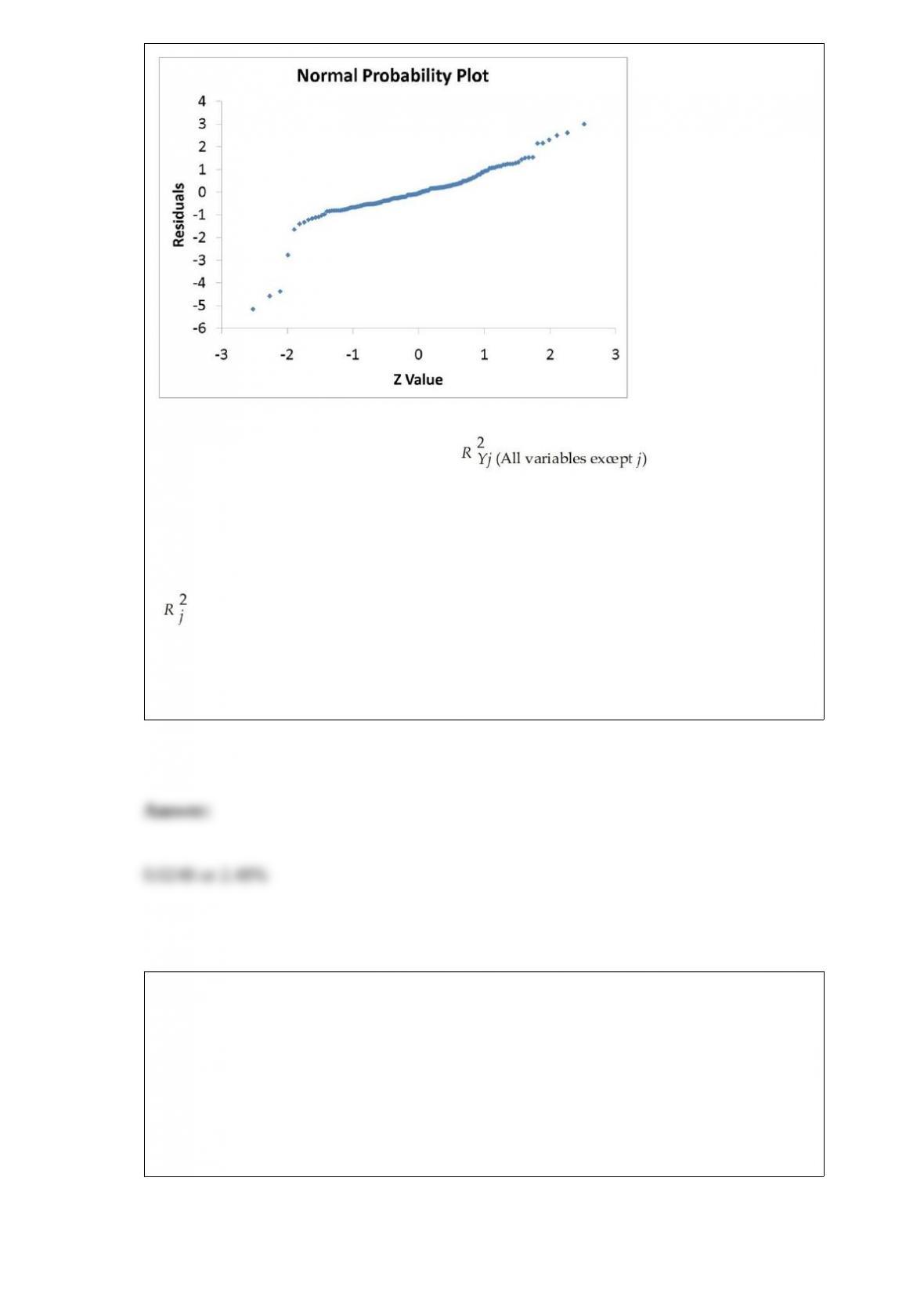
The coefficient of partial determination ( ) of each of the 5
predictors are, respectively, 0.0380, 0.4376, 0.0248, 0.0188, and 0.0312.
The coefficient of multiple determination for the regression model using each of the 5
variables Xj as the dependent variable and all other X variables as independent variables
( ) are, respectively, 0.7461, 0.5676, 0.6764, 0.8582, 0.6632.
Referring to Table 17-9, ________ of the variation in Accel Time can be explained by
MPG while controlling for the other independent variables.
TABLE 5-9
A major hotel chain keeps a record of the number of mishandled bags per 1,000
customers. In a recent year, the hotel chain had 4.06 mishandled bags per 1,000
customers. Assume that the number of mishandled bags has a Poisson distribution.
Referring to Table 5-9, what is the probability that in the next 1,000 customers, the
hotel chain will have more than ten mishandled bags?
You were told that the mean score on a statistics exam is 75 with the scores normally
distributed. In addition, you know the probability of a score between 55 and 60 is
4.41% and that the probability of a score greater than 90 is 6.68%. What is the
probability of a score between 60 and 75?
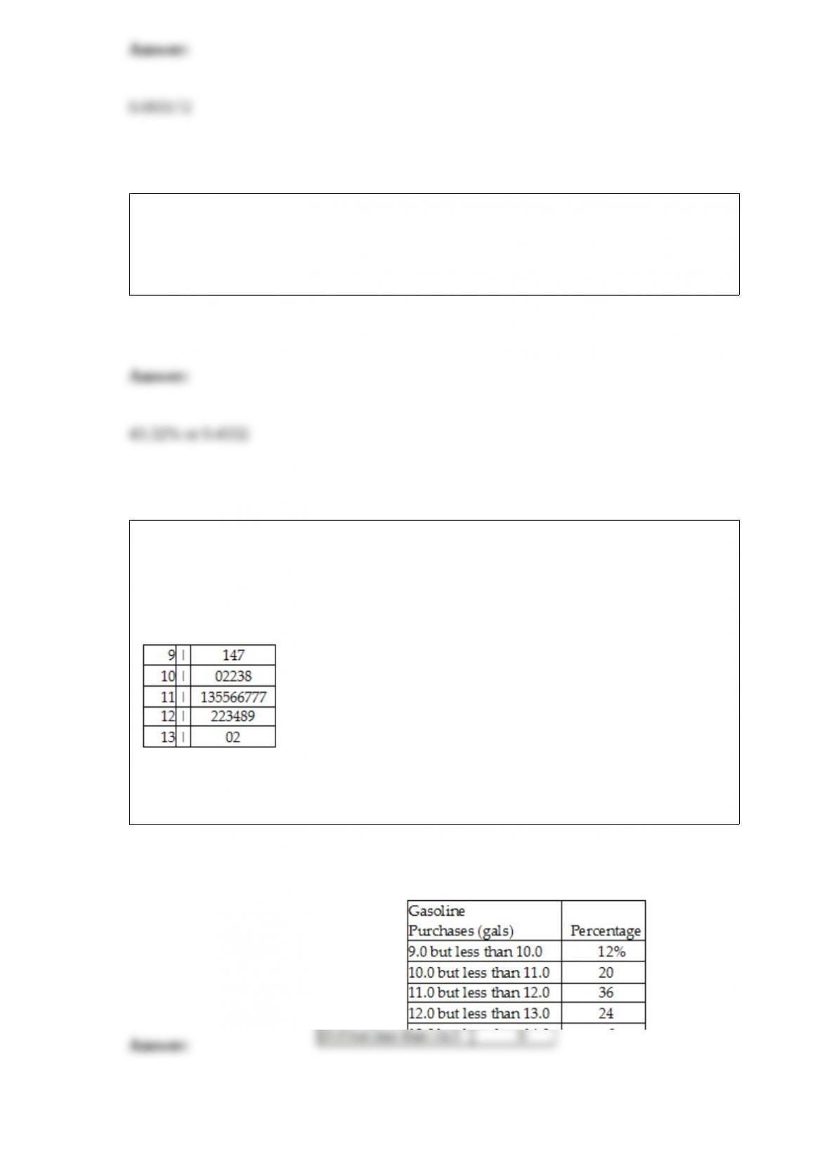
TABLE 2-13
Given below is the stem-and-leaf display representing the amount of detergent used in
gallons (with leaves in 10ths of gallons) in a day by 25 drive-through car wash
operations in Phoenix.
Referring to Table 2-13, construct a relative frequency or percentage distribution for the
detergent data, using “9.0 but less than 10.0” as the first class.

TABLE 3-4
The ordered array below represents the number of cargo manifests approved by customs
inspectors of the Port of New York in a sample of 35 days:
16, 17, 18, 18, 19, 20, 20, 21, 21, 21, 22, 22, 22, 22, 23, 23, 23, 23, 24, 24, 24, 25, 25,
26, 26, 26, 27, 28, 28, 29, 29, 31, 31, 32, 32
Note: For this sample, the sum of the values is 838, and the sum of the squared
differences between each value and the mean is 619.89.
Referring to Table 3-4, the range of the customs data is ________.