
TABLE 9-7
A major home improvement store conducted its biggest brand recognition campaign in
the company’s history. A series of new television advertisements featuring well-known
entertainers and sports figures were launched. A key metric for the success of television
advertisements is the proportion of viewers who “like the ads a lot”. A study of 1,189
adults who viewed the ads reported that 230 indicated that they “like the ads a lot.” The
percentage of a typical television advertisement receiving the “like the ads a lot” score
is believed to be 22%. Company officials wanted to know if there is evidence that the
series of television advertisements are less successful than the typical ad (i.e. if there is
evidence that the population proportion of “like the ads a lot” for the company’s ads is
less than 0.22) at a 0.01 level of significance.
True or False: Referring to Table 9-7, the company officials can conclude that there is
sufficient evidence to show that the series of television advertisements are less
successful than the typical ad using a level of significance of 0.05.
True or False: The coefficient of multiple determination is calculated by taking the ratio
of the regression sum of squares over the total sum of squares (SSR/SST) and
subtracting that value from 1.
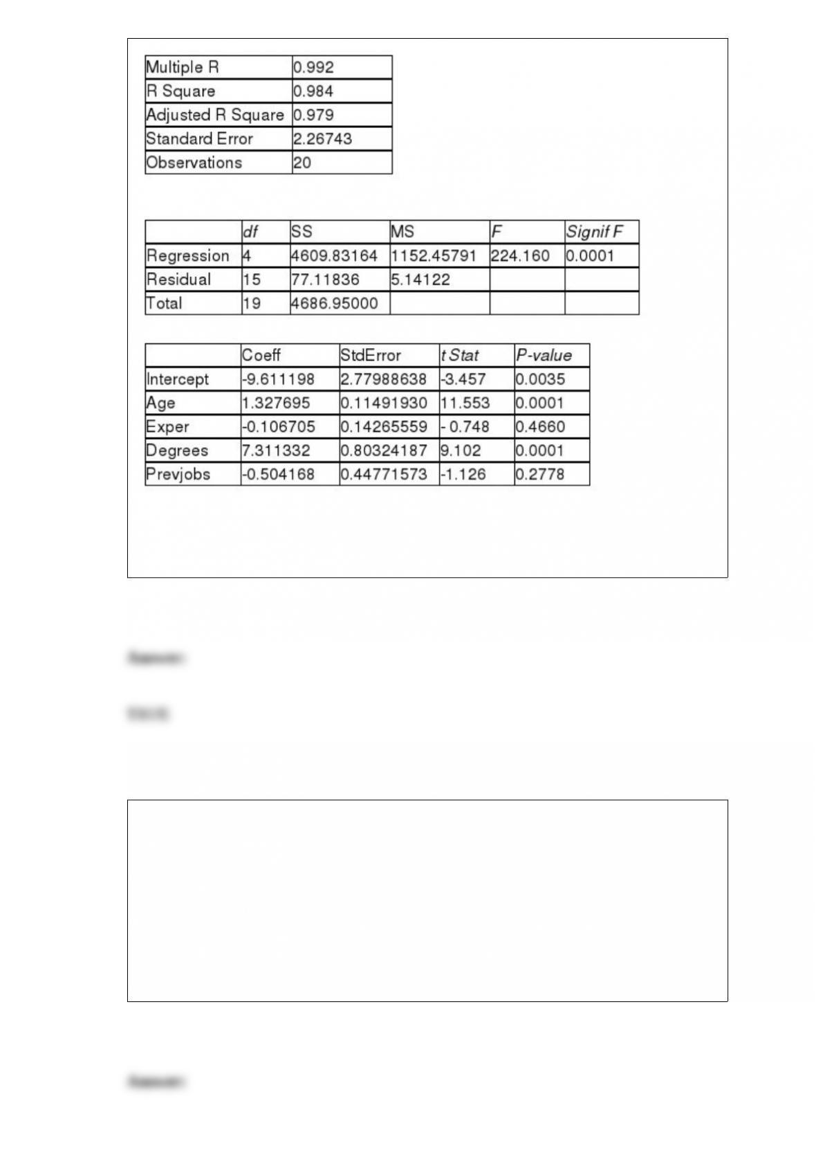
True or False: TABLE 17-3
A financial analyst wanted to examine the relationship between salary (in $1,000) and 4
variables: age (X1 = Age), experience in the field (X2 = Exper), number of degrees (X3 =
Degrees), and number of previous jobs in the field (X4 = Prevjobs). He took a sample of
20 employees and obtained the following Microsoft Excel output:
SUMMARY OUTPUT
Regression Statistics
ANOVA
Referring to Table 17-3, the analyst wants to use a t test to test for the significance of
the coefficient of X3. At a level of significance of 0.01, the department head would
decide that β3 ≠0.
TABLE 8-6
After an extensive advertising campaign, the manager of a company wants to estimate
the proportion of potential customers that recognize a new product. She samples 120
potential consumers and finds that 54 recognize this product. She uses this sample
information to obtain a 95% confidence interval that goes from 0.36 to 0.54.
True or False: Referring to Table 8-6, 95% of the time, the proportion of people that
recognize the product will fall between 0.36 and 0.54.
True or False: If a simple random sample is chosen with replacement, each individual
has the same chance of selection on every selection.
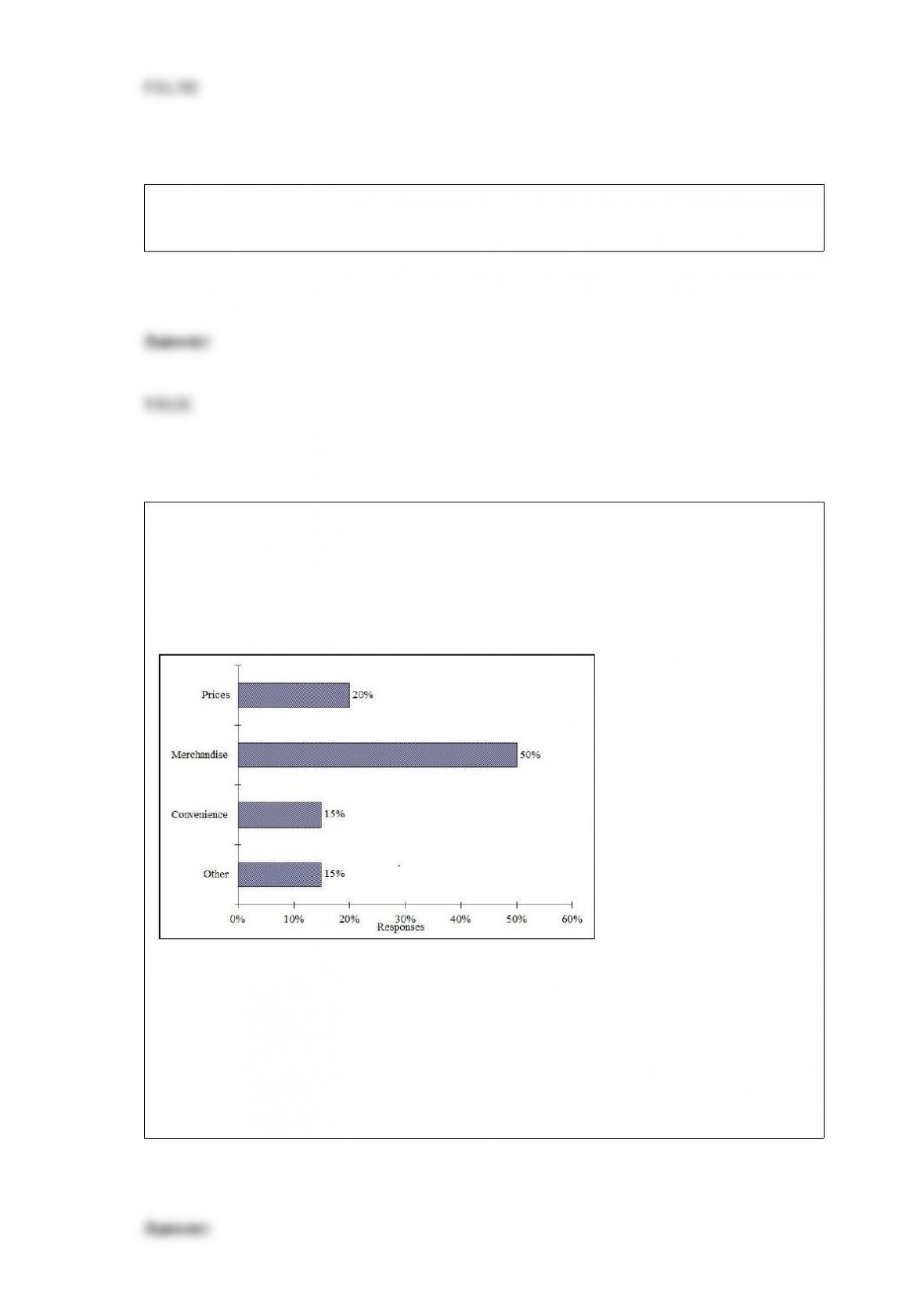
Retailers are always interested in determining why a customer selected their store to
make a purchase. A sporting goods retailer conducted a customer survey to determine
why its customers shopped at the store. The results are shown in the bar chart below.
What proportion of the customers responded that they shopped at the store because of
the merchandise or the convenience?
A) 35%
B) 50%
C) 65%
D) 85%

TABLE 1-1
The manager of the customer service division of a major consumer electronics company
is interested in determining whether the customers who have purchased a Blu-ray
player made by the company over the past 12 months are satisfied with their products.
Referring to Table 1-1, the possible responses to the question “What was your age at
your last birthday?” result in
A) a nominal scale variable.
B) an ordinal scale variable.
C) an interval scale variable.
D) a ratio scale variable.
A confidence interval was used to estimate the proportion of statistics students who are
female. A random sample of 72 statistics students generated the following 90%
confidence interval: (0.438, 0.642). Using the information above, what total size sample
would be necessary if we wanted to estimate the true proportion to within 0.08 using
95% confidence?
A) 105
B) 150
C) 420
D) 597
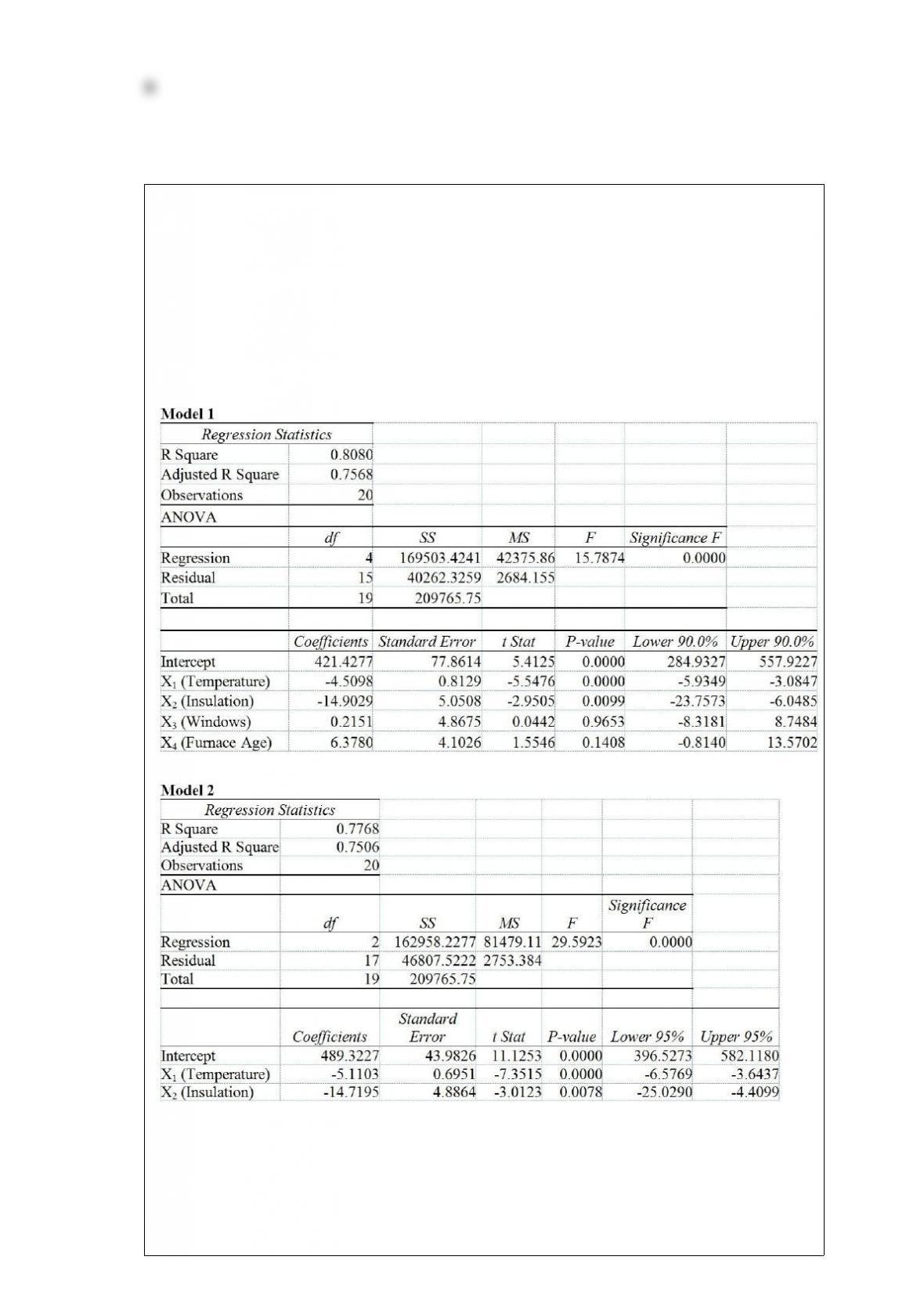
TABLE 17-2
One of the most common questions of prospective house buyers pertains to the cost of
heating in dollars (Y). To provide its customers with information on that matter, a large
real estate firm used the following 4 variables to predict heating costs: the daily
minimum outside temperature in degrees of Fahrenheit (X1), the amount of insulation in
inches (X2), the number of windows in the house (X3), and the age of the furnace in
years (X4). Given below are the EXCEL outputs of two regression models.
Referring to Table 17-2 and allowing for a 1% probability of committing a type I error,
what is the decision and conclusion for the test H0 : β1 = β2 = β3 = β4 = 0 vs. H1 : At
least one βj ≠0, j = 1, 2, …, 4 using Model 1?
A) Do not reject H0 and conclude that the 4 independent variables have significant
individual linear effects on heating costs.
B) Reject H0 and conclude that the 4 independent variables taken as a group have
significant linear effects on heating costs.
C) Do not reject H0 and conclude that the 4 independent variables taken as a group do
not have significant linear effects on heating costs.
D) Reject H0 and conclude that the 4 independent variables taken as a group do not
have significant linear effects on heating costs.
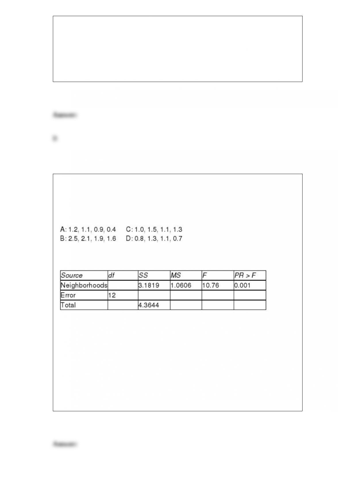
TABLE 11-2
A realtor wants to compare the mean sales-to-appraisal ratios of residential properties
sold in four neighborhoods (A, B, C, and D). Four properties are randomly selected
from each neighborhood and the ratios recorded for each, as shown below.
Interpret the results of the analysis summarized in the following table:
Referring to Table 11-2, what should be the conclusion for the Levene’s test for
homogeneity of variances at a 5% level of significance?
A) There is insufficient evidence that the variances are all the same.
B) There is sufficient evidence that the variances are all the same.
C) There is insufficient evidence that the variances are not all the same.
D) There is sufficient evidence that the variances are not all the same.

A supplier of silicone sheets for producers of computer chips wants to evaluate her
manufacturing process. She takes sample sizes of 5 from each day’s output and counts
the number of blemishes on each silicone sheet for 20 days consecutive days. Which of
the following would be the most appropriate analysis to perform?
A) Autoregressive modeling
B) Exponential smoothing
C) Multiple linear regression
D) Construct a c chart
TABLE 1-2
A Wall Street Journal poll asked 2,150 adults in the United States a series of questions
to find out their view on the U.S. economy.
Referring to Table 1-2, the possible responses to the question “How would you rate the
condition of the U.S. economy with 1 = excellent, 2 = good, 3 = decent, 4 = poor, 5 =
terrible?” result in
A) a nominal scale variable.
B) an ordinal scale variable.
C) an interval scale variable.
D) a ratio scale variable.
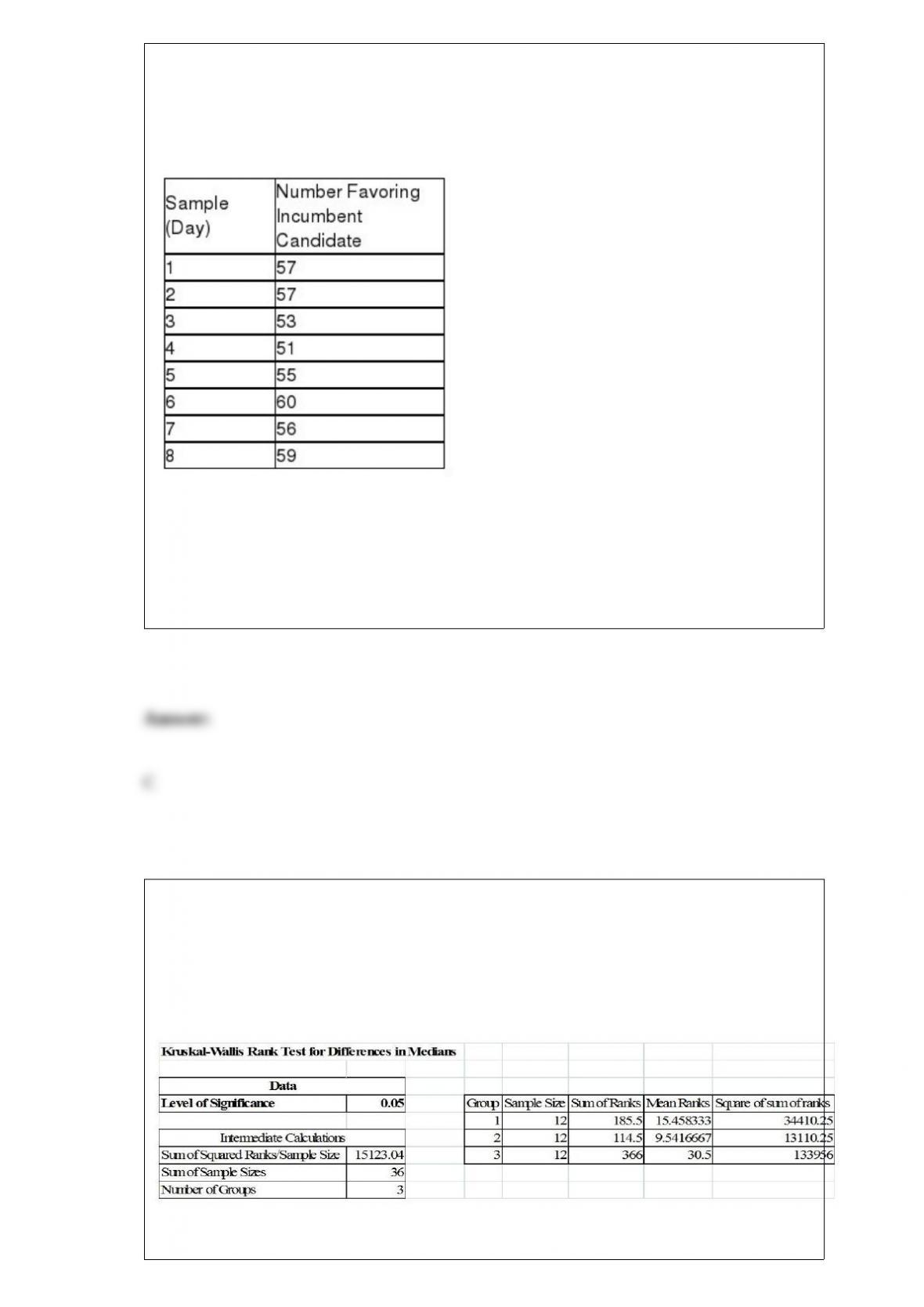
TABLE 18-2
A political pollster randomly selects a sample of 100 voters each day for 8 successive
days and asks how many will vote for the incumbent. The pollster wishes to construct a
p chart to see if the percentage favoring the incumbent candidate is too erratic.
Referring to Table 18-2, what is the numerical value of the upper control limit for the p
chart?
A) 0.92
B) 0.89
C) 0.71
D) 0.62
TABLE 12-17
Three new different models of compact SUVs have just arrived at the market. You are
interested in comparing the gas mileage performance of all three models to see if they
are the same. A partial computer output for twelve compact SUVs of each model is
given below:
You are told that the gas mileage population distributions for all three models are not

normally distributed.
Referring to Table 12-17, what should be the null and alternative hypotheses of the test?
A) H0: M1 = M2 = M3 vs. H1: M1M2M3
B) H0: M1 = M2 = M3 vs. H1: M1M2 = M3
C) H0: M1 = M2 = M3 vs. H1: M1 = M2M3
D) H0: M1 = M2 = M3 vs. H1: Not all Mj are equal (where j = 1, 2, 3)
Suppose a 95% confidence interval for turns out to be (1,000, 2,100). To make more
useful inferences from the data, it is desired to reduce the width of the confidence
interval. Which of the following will result in a reduced interval width?
A) Increase the sample size.
B) Increase the confidence level.
C) Increase the population mean.
D) Increase the sample mean.
Given the following information, calculate the degrees of freedom that should be used
in the pooled-variance t test.
s1
2 = 4 s2
2 = 6
n1 = 16 n2 = 25

A) df = 41
B) df = 39
C) df = 16
D) df = 25
A university dean is interested in determining the proportion of students who receive
some sort of financial aid. Rather than examine the records for all students, the dean
randomly selects 200 students and finds that 118 of them are receiving financial aid.
The 95% confidence interval for is 0.59 0.07. Interpret this interval.
A) We are 95% confident that the true proportion of all students receiving financial aid
is between 0.52 and 0.66.
B) 95% of the students get between 52% and 66% of their tuition paid for by financial
aid.
C) We are 95% confident that between 52% and 66% of the sampled students receive
some sort of financial aid.
D) We are 95% confident that 59% of the students are on some sort of financial aid.
If the outcome of event A is not affected by event B, then events A and B are said to be
A) mutually exclusive.
B) independent.

C) collectively exhaustive.
D) None of the above.
TABLE 1-1
The manager of the customer service division of a major consumer electronics company
is interested in determining whether the customers who have purchased a Blu-ray
player made by the company over the past 12 months are satisfied with their products.
Referring to Table 1-1, the possible responses to the question “What brand of Blu-ray
player did you purchase?” are values from a
A) discrete numerical variable.
B) continuous numerical variable.
C) categorical variable.
D) table of random numbers.
Referring to Table 14-11, what is the experimental unit for this
analysis?
TABLE 14-11
A weight-loss clinic wants to use regression analysis to build a model
for weight loss of a client (measured in pounds). Two variables
thought to a&ect weight loss are client’s length of time on the

weight-loss program and time of session. These variables are
described below:
Y = Weight loss (in pounds)
X1 = Length of time in weight-loss program (in months)
X2 = 1 if morning session, 0 if not
Data for 25 clients on a weight-loss program at the clinic were
collected and used to /t the interaction model:
Y = β0 + β1X1 + β2X2 + β3X1X2 + ε
Output from Microsoft Excel follows:
A) a clinic
B) a client on a weight-loss program
C) a month
D) a morning, afternoon, or evening session
The process of using data collected from a small group to reach conclusions about a
large group is called
A) statistical inference.
B) DCOVA framework.
C) operational definition.
D) descriptive statistics.
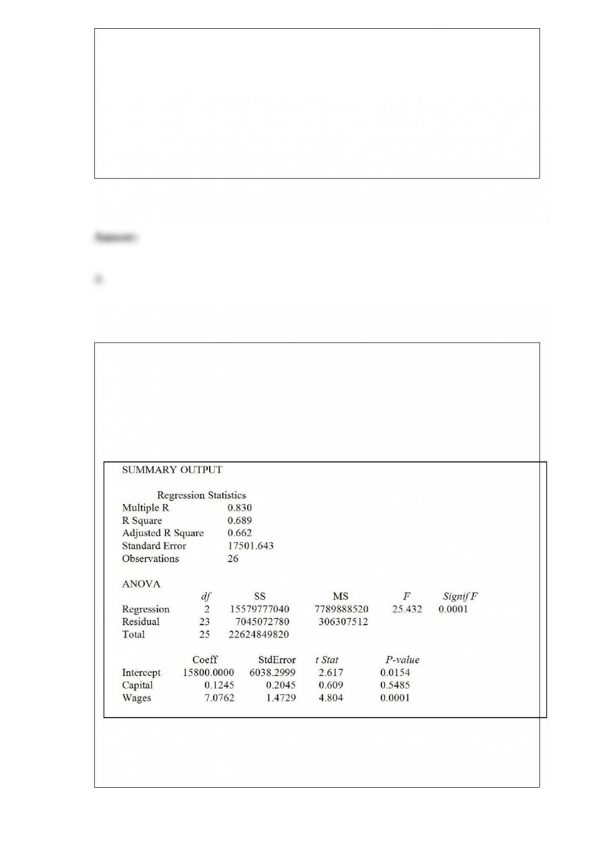
Referring to Table 14-5, what is the p-value for Wages?
TABLE 14-5
A microeconomist wants to determine how corporate sales are influenced by capital and
wage spending by companies. She proceeds to randomly select 26 large corporations
and record information in millions of dollars. The Microsoft Excel output below shows
results of this multiple regression.
A) 0.01
B) 0.05
C) 0.0001
D) None of the above

TABLE 1-2
A Wall Street Journal poll asked 2,150 adults in the United States a series of questions
to find out their view on the U.S. economy.
Referring to Table 1-2, the possible responses to the question “How many out of every
10 U.S. voters do you think feel that the U.S. economy is in good shape?” result in
A) a nominal scale variable.
B) an ordinal scale variable.
C) an interval scale variable.
D) a ratio scale variable.
TABLE 14-15
The superintendent of a school district wanted to predict the
percentage of students passing a sixth-grade proficiency test. She
obtained the data on percentage of students passing the proficiency
test (% Passing), mean teacher salary in thousands of dollars
(Salaries), and instructional spending per pupil in thousands of dollars
(Spending) of 47 schools in the state.
Following is the multiple regression output with Y = % Passing as the
dependent variable, X1 = Salaries and X2 = Spending:

Referring to Table 14-15, what is the value of the test statistic to
determine whether there is a signiticant relationship between
percentage of students passing the proficiency test and the entire set
of explanatory variables?
TABLE 4-8
According to the record of the registrar’s office at a state university, 35% of the students
are freshman, 25% are sophomore, 16% are junior and the rest are senior. Among the
freshmen, sophomores, juniors and seniors, the portion of students who live in the
dormitory are, respectively, 80%, 60%, 30% and 20%.
Referring to Table 4-8, what percentage of the students live in a dormitory?
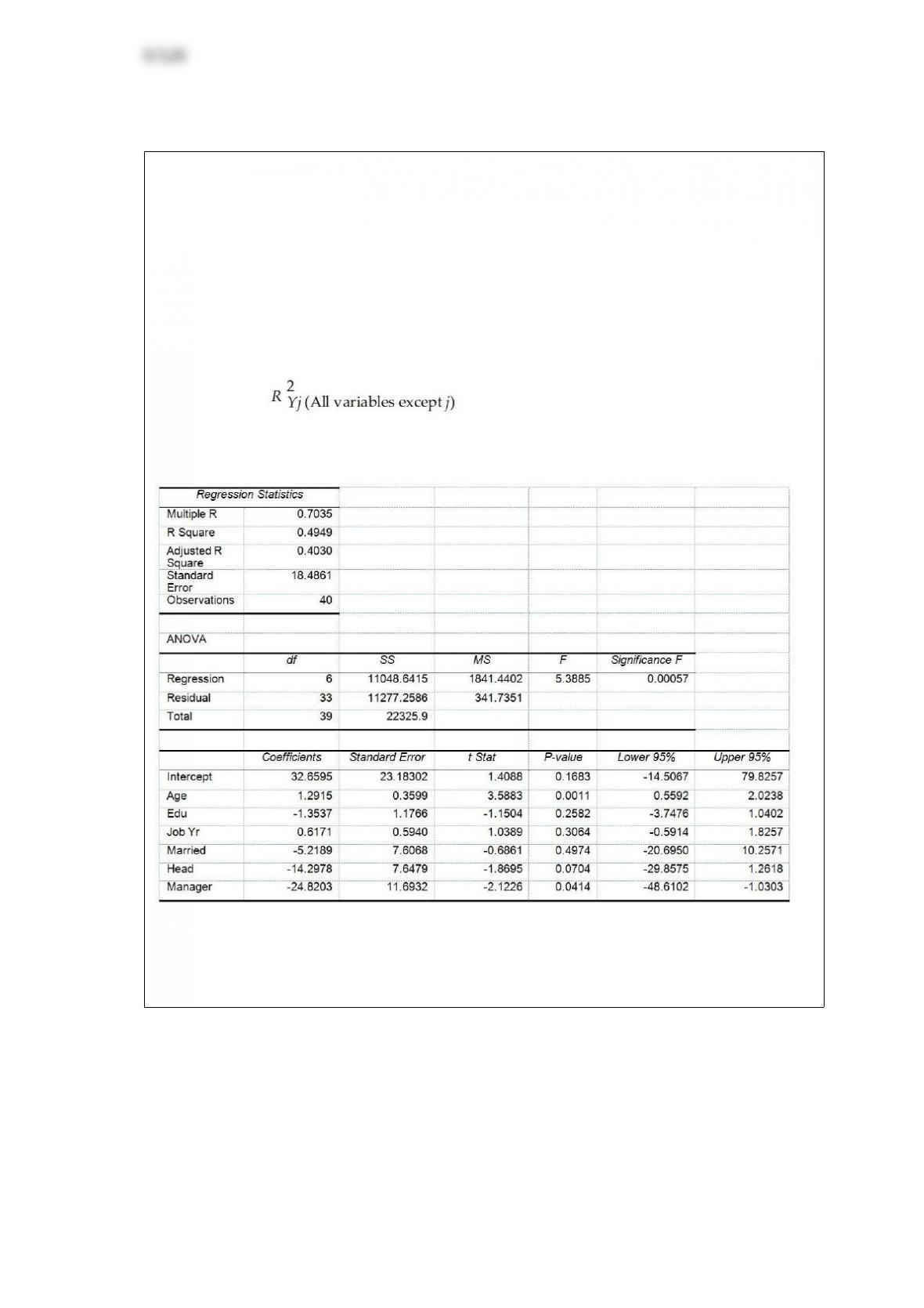
TABLE 17-10
Given below are results from the regression analysis where the dependent variable is
the number of weeks a worker is unemployed due to a layoff (Unemploy) and the
independent variables are the age of the worker (Age), the number of years of education
received (Edu), the number of years at the previous job (Job Yr), a dummy variable for
marital status (Married: 1 = married, 0 = otherwise), a dummy variable for head of
household (Head: 1 = yes, 0 = no) and a dummy variable for management position
(Manager: 1 = yes, 0 = no). We shall call this Model 1. The coefficient of partial
determination ( ) of each of the 6 predictors are, respectively,
0.2807, 0.0386, 0.0317, 0.0141, 0.0958, and 0.1201.
Model 2 is the regression analysis where the dependent variable is Unemploy and the
independent variables are Age and Manager. The results of the regression analysis are
given below:
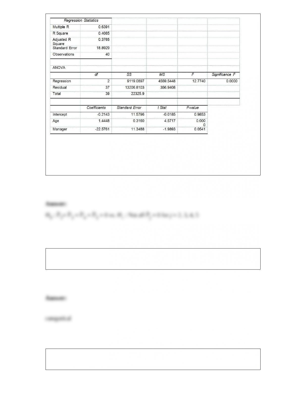
Referring to Table 17-10 and using both Model 1 and Model 2, what are the null and
alternative hypotheses for testing whether the independent variables that are not
significant individually are also not significant as a group in explaining the variation in
the dependent variable at a 5% level of significance?
A personal computer user survey was conducted. Primary word processing package
used is an example of a ________ variable.
The value that separates a rejection region from a non-rejection region is called the
________.
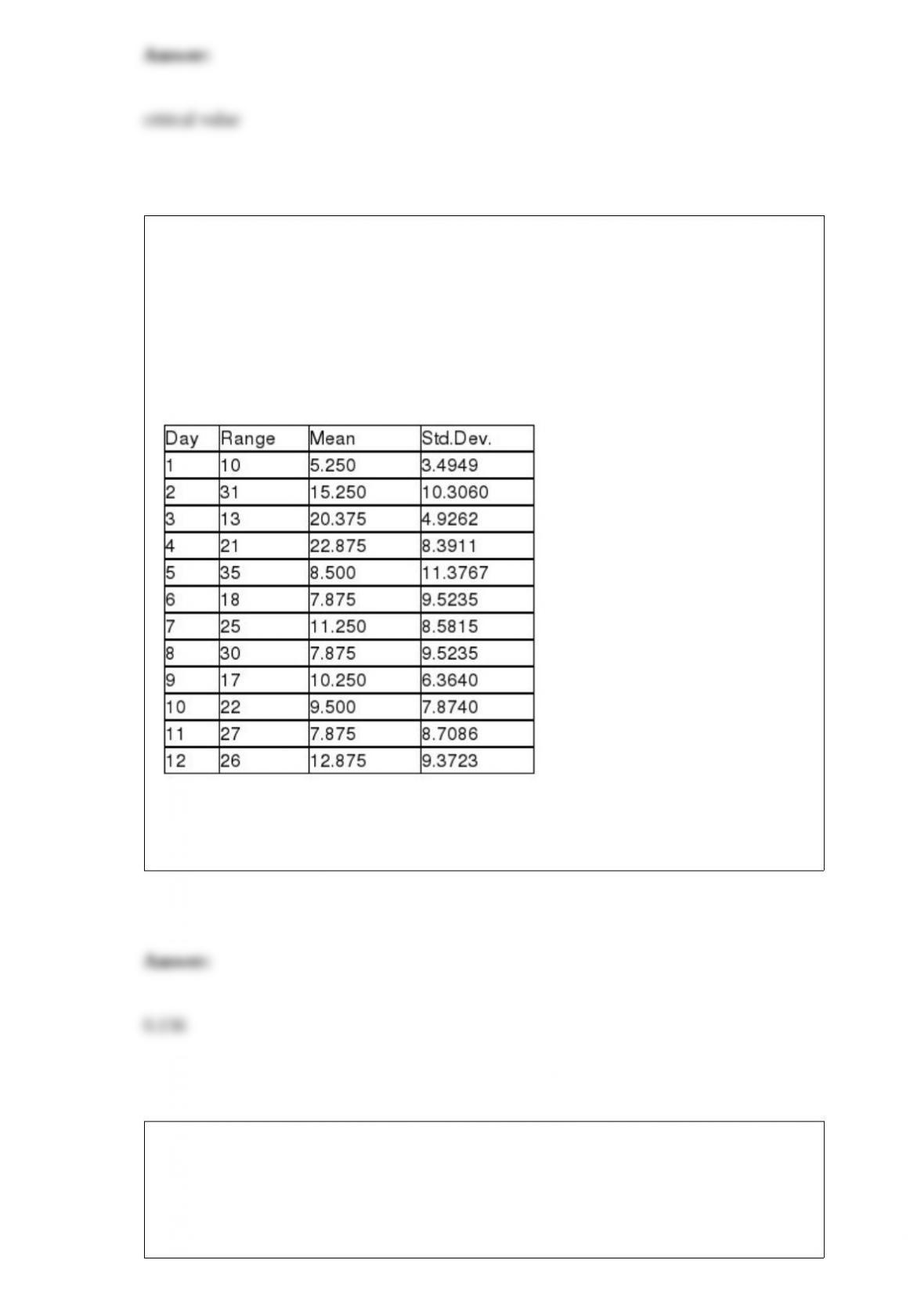
TABLE 18-8
Recently, a university switched to a new type of computer-based registration. The
registrar is concerned with the amount of time students are spending on the computer
registering under the new system. She decides to randomly select 8 students on each of
the 12 days of the registration and determine the time each spends on the computer
registering. The range, mean, and standard deviation of the times required to register are
in the table that follows.
Referring to Table 18-8, an R chart is to be constructed for the time required to register.
One way to create the lower control limit involves multiplying the mean of the sample
ranges by D3. For this data set, the value of D3 is ________.
TABLE 6-2
John has two jobs. For daytime work at a jewelry store he is paid $15,000 per month,
plus a commission. His monthly commission is normally distributed with a mean of
$10,000 and a standard deviation of $2,000. At night he works occasionally as a waiter,

for which his monthly income is normally distributed with a mean of $1,000 and a
standard deviation of $300. John’s income levels from these two sources are
independent of each other.
Referring to Table 6-2, for a given month, what is the probability that John’s income as
a waiter is more than $900?
Referring to Table 14-8, the value of the adjusted coefficient of
multiple determination is ________.TABLE 14-8
A financial analyst wanted to examine the relationship between salary
(in $1,000) and 2 variables: age
(X1 = Age) and experience in the field (X2 = Exper). He took a sample
of 20 employees and obtained the following Microsoft Excel output:
Also, the sum of squares due to the regression for the model that
includes only Age is 5022.0654 while the sum of squares due to the
regression for the model that includes only Exper is 125.9848.

TABLE 6-2
John has two jobs. For daytime work at a jewelry store he is paid $15,000 per month,
plus a commission. His monthly commission is normally distributed with a mean of
$10,000 and a standard deviation of $2,000. At night he works occasionally as a waiter,
for which his monthly income is normally distributed with a mean of $1,000 and a
standard deviation of $300. John’s income levels from these two sources are
independent of each other.
Referring to Table 6-2, the probability is 0.75 that John’s commission from the jewelry
store is less than how much in a given month?
TABLE 15-6
Given below are results from the regression analysis on 40 observations where the
dependent variable is the number of weeks a worker is unemployed due to a layoff (Y)
and the independent variables are the age of the worker (X1), the number of years of
education received (X2), the number of years at the previous job (X3), a dummy variable
for marital status (X4: 1 = married, 0 = otherwise), a dummy variable for head of
household (X5: 1 = yes, 0 = no) and a dummy variable for management position (X6: 1
= yes, 0 = no).
The coefficient of multiple determination ( ) for the regression model using each of
the 6 variables Xj as the dependent variable and all other X variables as independent
variables are, respectively, 0.2628, 0.1240, 0.2404, 0.3510, 0.3342 and 0.0993.
The partial results from best-subset regression are given below:
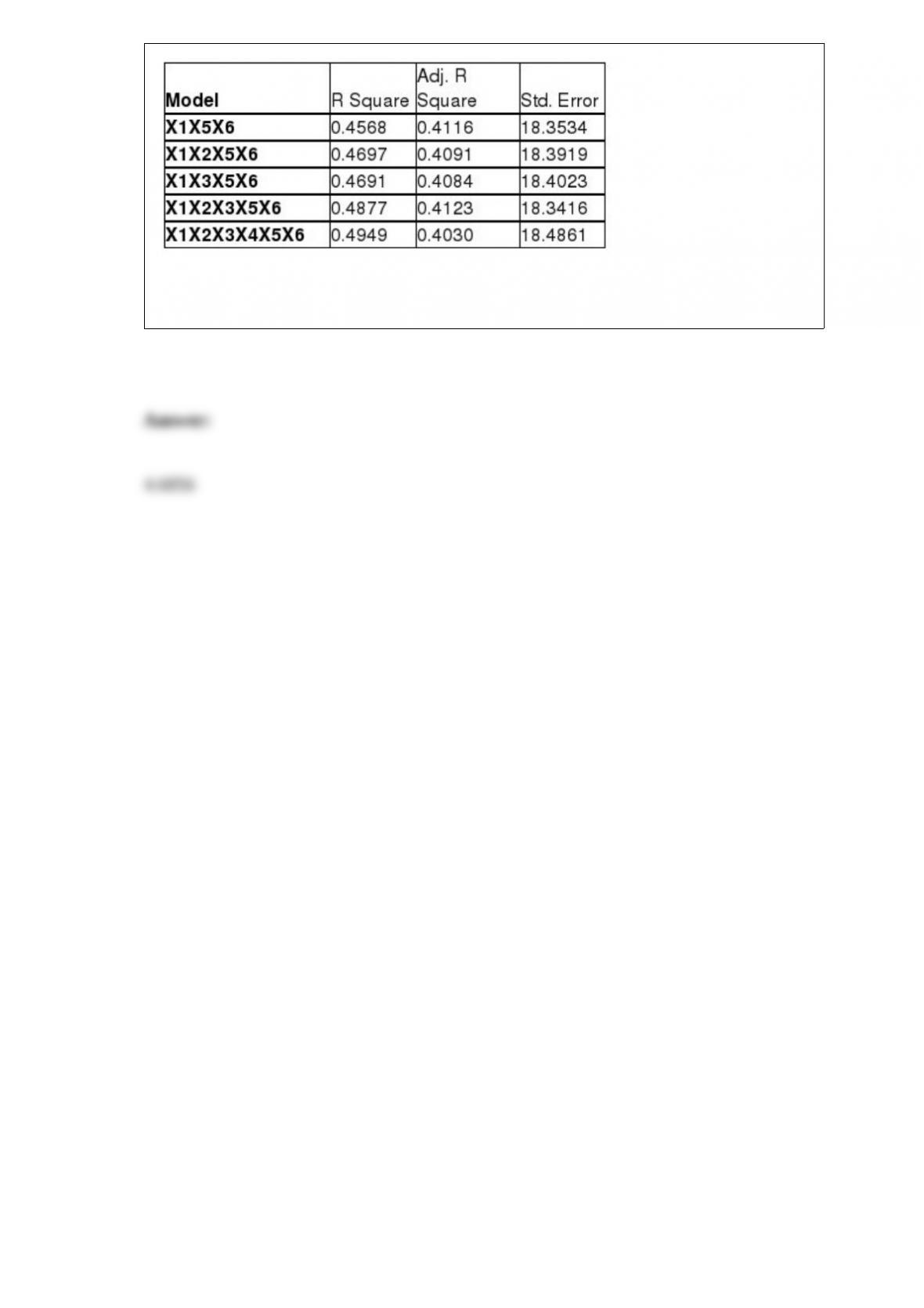
Referring to Table 15-6, what is the value of the Mallow’s Cp statistic for the model that
includes X1, X3, X5 and X6?