McDaniel & Gates – Marketing Research, 9th Edition Instructor’s Manual
CHAPTER 17
Bivariate Correlation and Regression
LEARNING OBJECTIVES
1. To comprehend the nature of correlation analysis.
3. To become aware of the coefficient of determination R2.
KEY TERMS
Bivariate regression analysis
Pearson’s product moment correlation
CHAPTER SCAN
This chapter examines the elements of bivariate analysis of association. Bivariate techniques are
statistical methods of analyzing the relationship between two variables, independent variables
and dependent variables. The bivariate regression is presented. If the data appears to be linear
when plotted on a scatter plot, regression can be used. An example is then used to explore the
CHAPTER OUTLINE
1. Bivariate Analysis of Association
I. Degrees of Association between Variables
2. Bivariate Regression
I. Bivariate Regression Analysis
3. Correlation Analysis
4. Summary
CHAPTER SUMMARY
1. BIVARIATE ANALYSIS OF ASSOCIATION
1. Bivariate Techniques–Statistical methods of analyzing the relationship between two
variables
3. Independent Variable (Predictor)–the symbol or concept that the researcher has some
4. Dependent Variable–a symbol or concept expected to be explained or caused by the
independent variable
B. Procedures for Metric and Ordinal Data
1. Metric Data
a. Bivariate Regression
2. Other Statistical Procedures

McDaniel & Gates – Marketing Research, 9th Edition Instructor’s Manual
2. BIVARIATE REGRESSION
I. Bivariate Regression Analysis
A. Bivariate Regression Analysis Defined–a statistical procedure which analyzes the strength
of the linear relationship between two variables when one is considered the independent variable
and the other the dependent variable
B. Nature of the Relationship
1. Scatter Diagram–one way to study the nature of the relationship between the dependent and
the independent variable is to plot the data in a scatter diagram
a. Dependent Variable Y–plotted on the vertical axis
b. Independent Variable X–plotted on the horizontal axis
c. Linear Relationship–apply linear regression to the data
d. Nonlinear Relationship–apply curve-fitting nonlinear regression techniques
See Exhibit 17.1 Types of Relationships Found in Scatter Diagrams (p 515)
C. Example of Bivariate Regression
2. Goal is to develop a model that can be used to evaluate potential sites for store locations.
4. A scatter plot of the resulting data was drawn.
See Exhibit 17.2 Annual Sales and Average Daily Vehicular Traffic (p 517).
Note: This example is used throughout most of the chapter as an illustration of how to utilize the
statistical tools discussed. .
See Practicing Marketing Research: Bivariate Regression Analysis Shows Higher Cancer
Rates among California Farm Workers (p 569)
Bivariate regression is a valuable statistical tool that is used widely in many fields, including
medicine. Recently, epidemiologists with the Cancer Registry of Central California in Fresno

McDaniel & Gates – Marketing Research, 9th Edition Instructor’s Manual
Discussion Questions
1. Are there other ways to configure this experiment in terms of which factors are the dependent
and independent variables?
2. How would you structure the bivariate correlation to handle different volumes of the
pesticides applied during the same time period?
See Exhibit 17.3 Scatterplot of Annual Sales by Traffic (p 518)
1. Least Squares Estimation Procedure
a. The least squares procedure is a simple mathematical technique that can be used to fit a line to
data for X and Y that best represents the relationship between the two variables.
b. No straight line will perfectly represent every observation in the scatterplot. This is reflected
in discrepancies between the actual values (dots on the scatter diagram) and predicted values
a
ˆ
b
ˆ
See Exhibit 17.4 Least Squares Computation (p 519)
See SPSS Jump Start for Regression (p 520)
2. Regression Line–Predicted values for Y, based on calculated values for
a
ˆ
and
b
ˆ
(Exhibit
17.5). In addition, errors for each observation
)Y
ˆ
Y( −
are shown. The regression line resulting
from the
Y
ˆ
values is plotted in Exhibit 17.6.
McDaniel & Gates – Marketing Research, 9th Edition Instructor’s Manual
See Exhibit 17 6 Least-Squares Regression Line Fitted to Sample Data (p 522)
3. Strength of Association – the estimated regression function describes the nature of the
relationship between the variables X and Y.
a. Coefficient of determination– denoted R2, measures strength of the linear relationship
between X and Y.
1) Indicates the percentage of the total variation in Y that is “explained” by the variation in X.
4. Statistical Significance of Regression Results
2) Error sum of squares (ESS)–variation not explained by the regression
See Exhibit 17.7 Measures of Variation in a Regression (p 524)
5. Hypotheses Concerning Overall Regression
The interest is in the hypotheses regarding the computed R2 value for the problem. Is the amount
of variance explained in the result significantly greater than should be expected due to chance?
Analysis of variance (an F test) is used to test the significance of the results
a. The null hypothesis H0–there is no linear relationship between X (average daily vehicular
traffic) and Y (annual sales).
b. Alternative hypothesis Ha–there is a linear relationship between X and Y.
d. F =MSR/MSE
e. Compare the calculated F-value to the table value of F.
f. Because the calculated F-value is > than the table value of F, reject the null hypothesis.
See Exhibit 17.8 Analysis of Variance (p 525)
See Exhibit 17.9 Regression Analysis Output (p 526)
1) Null hypothesis H0: b = 0
McDaniel & Gates – Marketing Research, 9th Edition Instructor’s Manual
2) Alternative hypothesis Ha: b ≠ 0
3. CORRELATION ANALYSIS
I. Correlation for Metric Data: Pearson’s Product Moment Correlation
A. Analysis between Two Variables
1. Correlation Defined–degree to which changes in one variable (the dependent variable) are
associated with the changes in another
a. Correlation Analysis Defined–analysis of the degree to which changes in one variable are
associated with changes in another
b. Pearson’s Product Moment Correlation–correlation analysis technique for use with metric
data
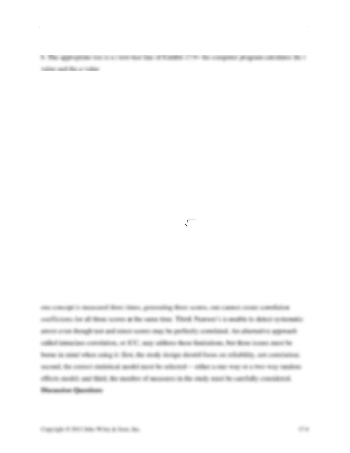
2. Coefficient of Correlation–R, is a measure of the degree of association between X and Y. It is
the square root of the coefficient of determination. It can range from –1(perfect negative
correlation) to +1(perfect positive correlation).
2
RR =
See Global Research: Rethinking the Applicability of Pearson’s Product–Moment
Correlation (p 527)
Using the Pearson correlation to calculate the reliability of results from test to retest has three
limitations. First, Pearson’s calculation is designed to show the relationship between two
variables, but it is inappropriate to apply this correlation to two data sets from the same variable.
Second, when multiple tests are employed, it’s hard to discern variations from test to test; when
2. Why is Pearson’s correlation unable to accurately reflect systematic errors, and how does ICC
better accommodate this function?
See SPSS Jump Start for Correlation (p 528-529)
See Global Research: Pearson’s Product–Moment Correlation Fine-Tunes Medical
Statistics (p 530-531)
Researchers in many fields, including medicine, rely on Pearson’s product–moment correlation
to fine-tune their analysis. For example, researchers at the Human Performance Laboratory and
Department of Internal Medicine at Vrije Universiteit Brussel in Brussels, Belgium assembled a
Discussion Questions
1. Explain the statistical operating principle that accounts for Pearson’s ability to clearly show
differences between the two groups as reflected in the r values.
2. Is there an r value, possibly on the high side, that would seem suspect if reported for this
study?
See Practicing Marketing Research: When Bivariate and Multivariate Correlation
Combined Give the Best Picture (p 531-532)
Social researchers, Kirby, Coyle, and Gould wanted to assess the relationships between
4. SUMMARY
QUESTIONS FOR REVIEW AND CRITICAL THINKING
1. Give an example of a marketing problem for which each of the two procedures covered
in the chapter would be appropriate.
Student answers may vary.
2. A sales manager of a life insurance firm administered a standard multiple-item job
satisfaction scale to all the members of the firm’s sales force. The manager then correlated
(Pearson’s product-moment correlation) job satisfaction score with years of school
completed for each salesperson. The resulting correlation was .11. On the basis of this
evidence, the sales manager concluded: “A salesperson’s level of education has little to do
with his or her job satisfaction.” Would you agree or disagree with this conclusion?
Explain the basis for your answer.
3. What purpose does a scatter diagram serve?
A scatter diagram is used to plot data observations to determine if the relationship appears to be
4. Explain the meaning of the coefficient of determination. What does this coefficient tell
the researcher about the nature of the relationship between the dependent and independent
variables?
The coefficient of determination tells the marketing researcher how much variation in the
dependent variable can be explained by variation in the independent variable. It is a measure of
5. It has been observed in the past that when an AFC team wins the Super Bowl, the stock
market rises in the first quarter of the year in almost every case. When an NFC team wins
the Super Bowl, the stock market falls in the first quarter in most cases. Does this mean
that the direction of movement of the stock market is caused by which conference wins the
Super Bowl? What does this example illustrate?
6. The following table gives the data collected for a convenience store chain for 20 of its
stores.
Column 1 – ID number for each store
Column 2 – Annual sales for the store for the previous year in thousands of dollars.
Column 3 – Average number of vehicles that pass the store each day, based on actual traffic
counts for one month.
Answer the following:
a. Which of the other three variables is the best predictor of sales? Compute correlation
coefficients to answer the question.
• For the correlation between sales and traffic, r = .769
b. Do the following regressions.
1. Sales as a function of average daily traffic.
2. Sales as a function of population in two-mile radius.
c. Interpret the results of the two regressions.

7. Interpret the following:
a. Y = .11 + .009X, where Y is the likelihood of sending children to college and X is
family income in thousands of dollars. Remember, it is family income in thousands.
1. According to our model how likely is a family with an income of $100,000 to send their
children to college?
2. What is the likelihood for a family with an income of $50,000?
3. What is the likelihood for a family with an income of $17,500?
4. Is there some logic to the estimates? Explain.
b. Y = .25 – .039X, where Y is the likelihood of going to a skateboard park and X is
age.
1. According to our model, how likely is a 10 year old to go to a skateboard park?
2. What is the likelihood for a 60 year old?
3. What is the likelihood for a 40 year old?
4. Is there some logic to the estimates? Explain.
8. The following ANOVA summary data are the result of a regression with sales per year
(dependent variable) as a function of promotion expenditures per year (independent
variable) for a toy company.
The degrees of freedom are 1 for the numerator and 19 for the denominator. Is the
relationship statistically significant at α = .05? Comment.
With this summary data, we can compute an F-value of 7.26. With one and 19 degrees of
WORKING THE NET
1. For an informative and practical tutorial with examples and graphs on different
regression models with count data (including Poisson, negative binomial, zero-inflated
count models, and others), visit:
www.ats.ucla.edu/STAT/stata/seminars/count_presentation/count.htm
Experiences will vary
2. For a free online statistical calculator to work with the Pearson’s product–moment
correlation, see: www.wessa.net
3. Take a look at the video on correlation at http://www.youtube.com/ watch?v=Fd-
V9W7dK04.
Experiences will vary.
REAL-LIFE RESEARCH
Case 17.1 – Axcis Athletic Shoes
Key Points:
1. Which of the statistical procedures covered in this chapter is appropriate for addressing
Fred’s theory? Why would you choose that technique over the others?
Pearson’s product-moment correlation would be appropriate, as it is designed to quantify the
nature and strength of association between variables measured on metric scales. We could also
run bivariate regression if a predictive model is desired.
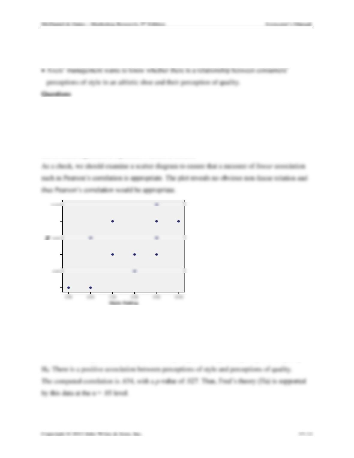
2. Use the technique that you choose to determine whether Fred’s theory is supported by
the statistical evidence. State the appropriate null and alternative hypothesis. Is Fred’s
theory supported by the statistical evidence? Why or why not?
Fred’s theory is represented by the alternative hypothesis in an inference test for the correlation.
H0: There is not a positive association between perceptions of style and perceptions of quality.
Quality Rating
9.00
7.00
5.00
Case 17.2 – The Carter Regional Blood Center
Key Points:
In the past, many small communities had their own blood programs and patients received whole
blood. It usually was organized by local hospital and civic leaders to meet the needs of the
1. Which of the other two variables is most closely associated with Pints Donated? Compute
correlation coefficients to answer the question.
2. Do the following regressions.
a. Amount donated as a function of Age.
b. Amount donated as a function of Education.
3. Interpret the results of the two regressions.
This will make an excellent in class excercise.
SPSS EXERCISES FOR CHAPTER 17
EXERCISE 1: Bivariate Regression
Use the analyze/regression/linear sequence to invoke bivariate regression analysis. This exercise
1. Q3 and Q5d (movie theater item – importance of comfortable chairs)
2. Q3 and Q5e (movie theater item – auditorium type seating)

3. Q3 and Q7a (movie theater information source – newspaper)
4. Q3 and Q7b (movie theater information source – Internet)
5. Q3 and Q7c (movie theater information source – phone in for information)
6. Q3 and Q9 (self perception of how physically active)
7. Q3 and Q10 (self-perception of how socially active)
Summarize the results of the bivariate regression analysis by filling in tables similar to the
ones below.
Model
Constant
Regression
coefficient
t-value for
coefficient
Sig.
Q5d
.71
.24
2.37
.02
Q5e
1.07
.15
2.05
.04
Q7a
1.68
-.04
-.62
.53
Q7b
1.43
.05
.75
.45
Q7c
1.20
.14
2.44
.02
Q9
1.31
.08
.97
.33
Q10
1.66
-.03
-.32
.75
Variables
R2
F–
value
Sig.
Q5d
.012
5.60
.02
.009
4.21
.04
.001
.53
Q7b
.001
.45
.013
5.94
.02
.002
.33
Q10
.000
.75
1. At the 95 percent level of confidence, which of the regression models (list the pairs of
variables) are significant?
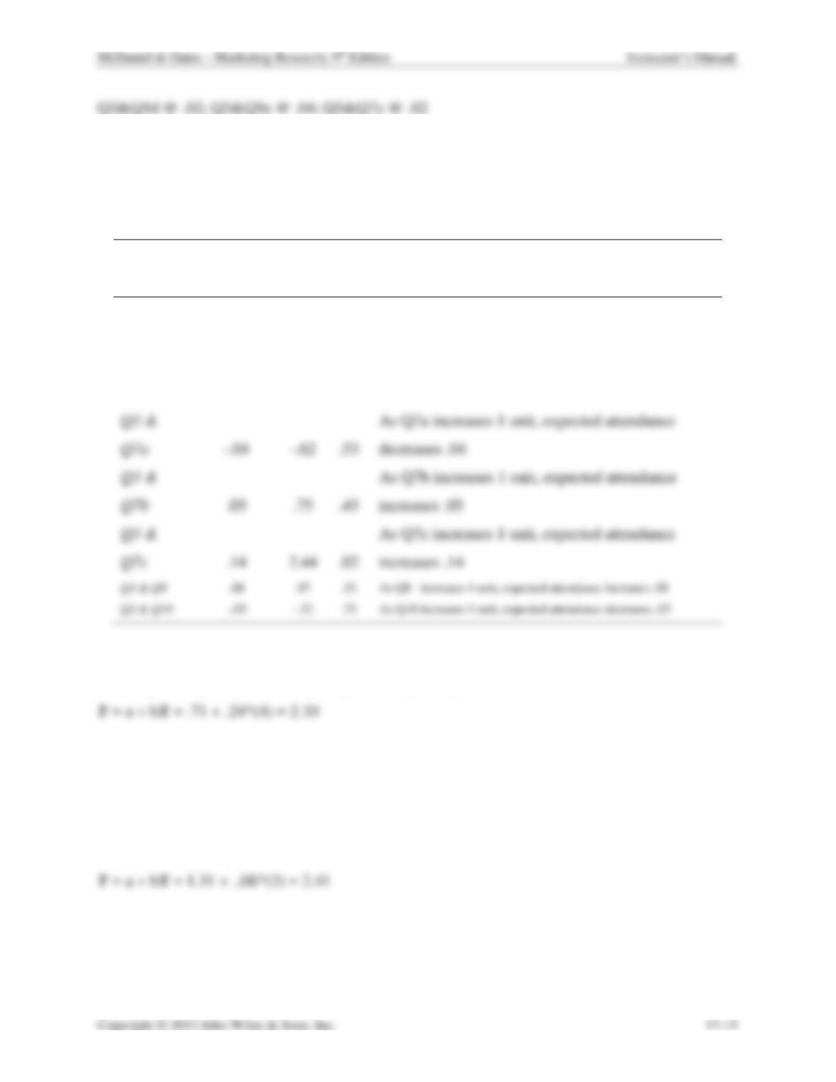
2. Interpretation of the regression coefficients: Use the following table to summarize the
regression coefficient, b in each of the 7 regression models.
Model
Regression
coefficient
t
Sig.
Interpretation of
Regression Coefficient
Q3 &
Q5d
.24
2.37
.02
As Q5d increases 1 unit, expected attendance
increases .24
Q3 &
Q5e
.15
2.05
.04
As Q5e increases 1 unit, expected attendance
increases .15
Q3 &
Q7a
.53
As Q7a increases 1 unit, expected attendance
decreases .04
Q3 &
Q7b
.05
.75
.45
As Q7b increases 1 unit, expected attendance
increases .05
3. Using the regression results, compute Y (Q3) if Q5d = 4.
4. Using the regression results, compute Y (Q3) if Q7c = 2.
Y = a + bX = .1.20 + .14*(2) = 2.30
5. Using the regression results, compute Y (Q3) if Q9 = 3.
6. Which of the 7 models in the bivariate regression analysis explained the most variation in
Q3 (Hint: R2)?
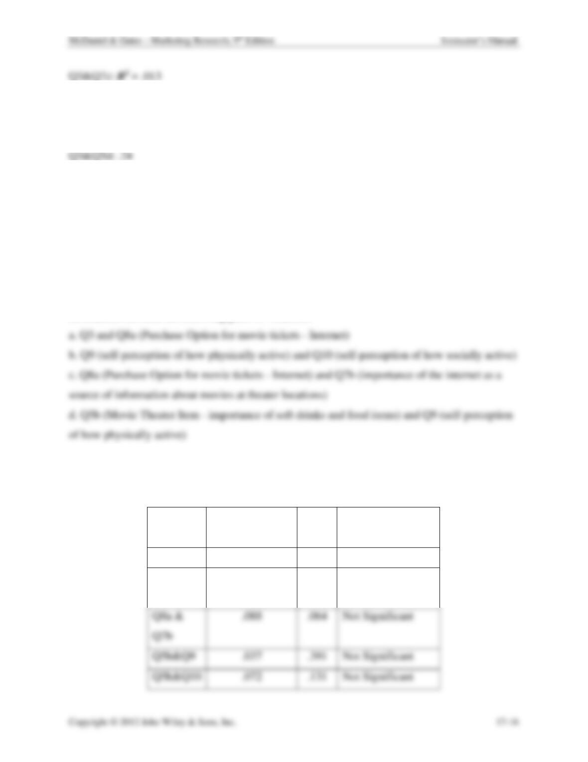
Q5b&Q9
.037
.391
Not Significant
Q5h&Q10
.072
.131
Not Significant
7. In which of the 7 models does the independent variable’s regression coefficient cause the
largest change in Q3 for a one-unit change in the independent variable?
EXERCISE 2: Pearson’s Product-Moment Correlation
Use the analysis/correlate/bivariate sequence to invoke bivariate correlation analysis. This
exercise utilizes the metric correlation technique (Pearson’s), which requires that both variables
in the bivariate analysis be of at least interval measurement scale. The objective of this exercise
is to examine the association between various pairs of variables.
Invoke the bivariate correlation procedure to utilize the Pearson coefficient to evaluate the
association between the following pairs of variables:
e. Q5h (Movie Theater Item – number of screens at a movie theater) and Q10 (self-perception of
how socially active) With the results of the bivariate correlation using the Pearson coefficient,
fill in a table similar to the one below.
Variables
Pearson
Coefficient
p-
value
Interpretation
Q3 & Q8a
.015
.748
Not Significant
Q9 & Q10
.415
.000
Significant at .01
level

McDaniel & Gates – Marketing Research, 9th Edition Instructor’s Manual
Questions to Answer: (Assume a significant relationship requires at least a 95 percent level
of confidence).
1. Of the five correlations computed, which pair of variables had the strongest association?
2. Of the five correlations computed, which pair of variables had the weakest association?
3. Do people who perceive themselves as more physically active have a greater or lesser
need for food and drink at a movie theater?
4. Are people who use the Internet to purchase movie tickets more or less likely to use the
Internet to get information about movies at movie theaters?