McDaniel & Gates – Marketing Research, 9th Edition Instructor’s Manual
Instructor’s Manual
because of chance. Managerial importance is the concept that the difference is large enough to
have meaning in the decision the manager makes.
2. Describe the steps in the procedure for testing hypotheses. Discuss the difference
between a null hypothesis and an alternative hypothesis.
In hypothesis testing, the first step is the state the hypothesis. The convention is to state the
generally accepted condition, or status quo, as the null hypothesis. Then the alternative
hypothesis is stated. The second step involves choosing the appropriate test statistic.
3. Distinguish between a Type I error and Type II error. What is the relationship between
the two?
Type I error, or alpha level, is the probability that the researcher will reject the null hypothesis
when it is actually true. Type II error, or beta error, is the probability that the researcher will fail
4. What is meant by the terms independent samples and related samples? Why is it
important for a researcher to determine whether an ample is independent?
Instructor’s Manual
An independent sample is a sample in which measuring a variable in one population has no
effect on measuring that variable in another population. An example would be determining the
5. Your university library is concerned about student desires for library hours on Sunday
morning (9:00 a.m. – 12:00 p.m.). It has undertaken a random sample of 1,600
undergraduate students (one-half men, one half women) in each of four status levels (i.e.
400 freshmen, 400 sophomores, 400 juniors, 400 seniors.) If the percentage of students
preferring Sunday morning hours are those shown below, what conclusions can the library
reach?
Observed Results
Sen
Jun
Soph
Fresh
TOTAL
Women
70
53
39
26
188
Men
30
48
31
27
136
TOTAL
100
101
70
53
324
STEP 1: Hypotheses
STEP 2: Determine Expected Results
Expected Results if the variables are independent*
Sen
Jun
Soph
Fresh
TOTAL
Women
58.02
58.60
40.62
30.75
188
Men
41.98
42.40
29.38
22.25
136
TOTAL
100
101
70
53
324
*Cell values calculated by multiplying each row margin total by each column margin total and
dividing by the grand total
STEP 3: Calculate Chi-Square Value
Chi-square Calculations*
Sen
Jun
Soph
Fresh
TOTAL
Men
3.42
0.74
0.09
1.02
TOTAL
2=
9.07
* Cell values calculated by taking the squared difference between the expected and observed and
dividing expected
STEP 4: Find Chi Square Table Value based on Significance Level and Degrees of Freedom
STEP 5: Compare Results and State Conclusion
The calculated chi square = 9.06
Conclusion: Calc 2 > Table 2
6. A local car dealer is attempting to determine which premium will draw the most visitors
to its showroom. An individual who visits the showroom and takes a test ride is given a
premium with no obligation. The dealer chose four premiums and offered each for one
week. The results are as follows:
Week
Premium
Total Given Out
1
Four-foot metal stepladder
425
2
$50 savings bond
610
3
Dinner for four at a local steakhouse
510
4
Six pink flamingos plus an outdoor thermometer
705
Using a chi-square test, what conclusions can be drawn regarding the premiums?
STEP 1: Hypotheses
Ho: The number of people visiting the showroom in response to different premiums is the same.
STEPS 2-3: Determine Expected Results and Calculate Chi-Square Value
Observed
Expected*
E-O
(E-O)2
(E-O)2/E
Promo 1
425
562.5
137.5
18906.25
33.61
Instructor’s Manual
Promo 4
705
562.5
-142.5
20306.25
36.10
TOTAL
78.62
STEP 4: Find Chi Square Table Value based on Significance Level and Degrees of Freedom
Degrees of freedom = (k-1) = (4-1) = 3
7. A market researcher has completed a study of pain relievers. The following table depicts
the brand purchased most often broken down by men versus women. Perform a Chi-
square test on the data and determine what can be said regarding the crosstabulation.
Pain Reliever Men Women
Pain Reliever
Men
Women
Anacin
40
55
Bayer
60
28
Bufferin
70
97
14
21
Empirin
82
107
Excedrin
72
84
Excedrin PM
15
11
Vanquish
20
STEP 1: Hypotheses
Ho: There is no relationship between gender and the type of brand purchased.
Ha: There is a significant relationship between gender and the type of brand purchased.
STEP 2: Determine Expected Results
Expected Results If the Variables Are Independent
Pain Reliever
Men
Women
Total
Anacin
44.18
50.82
95
Bayer
40.93
47.07
88
McDaniel & Gates – Marketing Research, 9th Edition Instructor’s Manual
Instructor’s Manual
Bufferin
77.67
89.33
167
Cope
16.28
18.72
35
Empirin
87.90
101.10
189
Excedrin
72.55
83.45
156
Vanquish
21.39
24.61
46
Total:
373
802
STEP 3: Calculate Chi-Square Value
Pain Reliever
Men
Women
Anacin
0.40
0.34
Bayer
8.89
7.73
Bufferin
0.76
0.66
Cope
0.32
0.28
Empirin
0.40
0.34
Excedrin
0.00
0.00
Excedrin PM
0.70
0.61
Vanquish
0.09
0.08
2=
21.59
STEP 4: Find Chi Square Table Value based on Significance Level and Degrees of Freedom
Degrees of freedom = (r-1) * (k-1) = (8-1) * (2-1) = 7
The tabulated chi square, 7 df, .05 alpha = 14.067
STEP 5: Compare Results and State Conclusion
The calculated Chi square = 21.59
8. A child psychologist observed 8-year-old children behind a one-way mirror to determine
how long they would play with a toy medical kit. The company that designed the toy was
attempting to determine whether to give the kit a masculine or feminine orientation. The
length of time (in minutes) the children played with the kits are shown below. Calculate the
value of Z and recommend to management whether the kit should have a male or female
orientation.
Instructor’s Manual
Sex
Time played with toy medical kit
Boys
31
12
41
34
63
7
67
67
25
73
36
41
15
Girls
26
38
20
32
16
45
9
9
16
26
81
20
5
STEP 1: Hypotheses
Ho: The difference in the means is less than or equal to zero; the mean length of time the toy
holds a boy’s attention is the same or less than the mean length of time the toy holds a girl’s
STEP 2: Decide on Significance Level and Look up Appropriate Table Value
Assume an alpha of 0.05. Since the sample size is less than 30, it is appropriate to use a t-test.
This is also a two tailed test, hence, the value from the t table for n=12 and alpha = 0.05 is 2.179
STEP 3: Calculate the Pooled Standard Error for the two samples
Sex
Time played with toy medical kit
Avg.
S
S2
S2/n
Boys
31
12
41
34
63
7
67
67
25
73
36
41
15
39.38
22.23
494.09
38.01
Girls
20
32
16
45
16
26
81
20
20.11
Observ.
10
11
12
13
STEP 4: Calculate the test statistic
The observed difference in the means is 13. Therefore the t-calculated is equal to 13/8.31 or 1.56
STEP 5: Compare Results and State Conclusion
9. American Airlines is trying to determine which baggage handling system it will put in its
new hub terminal at San Juan, Puerto Rico. One system is made by Jano Systems and a
second baggage handling system is manufactured by Dynamic Enterprises. American has
installed a small Jano system and a small Dynamic Enterprises system in two of its low-
volume terminals. Both terminals handle approximately the same quantity of baggage each
month. American has decided to select the system that will provide the minimum number
McDaniel & Gates – Marketing Research, 9th Edition Instructor’s Manual
Instructor’s Manual
of instances in which passengers disembarking must wait 20 minutes or longer for baggage.
Analyze the data that follow and determine whether there is a significant difference at the
.95 level of confidence between the two systems. If there is a difference, which one should
American select?
Minutes of Waiting
Jano Systems
(Frequency)
Dynamic Enterprise
(Frequency)
10-11
4
10
12-13
10
8
14-15
14
14
16-17
4
20
18-19
2
12
20-21
4
6
22-23
2
12
24-25
14
4
26-27
6
13
28-29
10
8
30-31
12
6
32-33
2
8
34-35
2
8
36 or more
2
2
STEP 1: Hypotheses and determine sample proportions
Ho: The difference in the proportions is less than or equal to zero; the proportion of those who
Number of People who waited 20 minutes
Instructor’s Manual
STEP 2: Decide on Significance Level and Look up Appropriate Table Value
Management wants a 95% confidence level, hence an alpha of 0.05. This is a two tailed test,
hence, the value from the Z table for alpha = 0.05 is +/-1.96.
STEP 3: Calculate the Pooled Standard Error for the two proportions
Hence, the pooled standard error of the proportions equals .069
STEP 4: Calculate the test statistic
STEP 5: Compare Results and State Conclusion
Since Zcalc =1.49 < Ztable=1.96, we conclude there is no statistical difference between the
proportions.
10. Menu space is always limited in fast food restaurants. However, McDonald’s has
decided that it needs to add one more salad dressing to its menu for its garden salad and
check salad. It has decided to test market four flavors: Caesar, Ranch-style, Green
Goddess, and Russian. Fifty restaurants were selected in the North-Central region to sell
each new dressing. Thus, a total of 200 stores were used in the research project. The study
was conducted for two weeks and the units of each dressing sold are shown below. As a
researcher, you want to know if the differences among the average daily sales of the
dressings are larger than can be reasonably expected due to chance. If so, which dressing
would you recommend be added to the inventory throughout the United States?
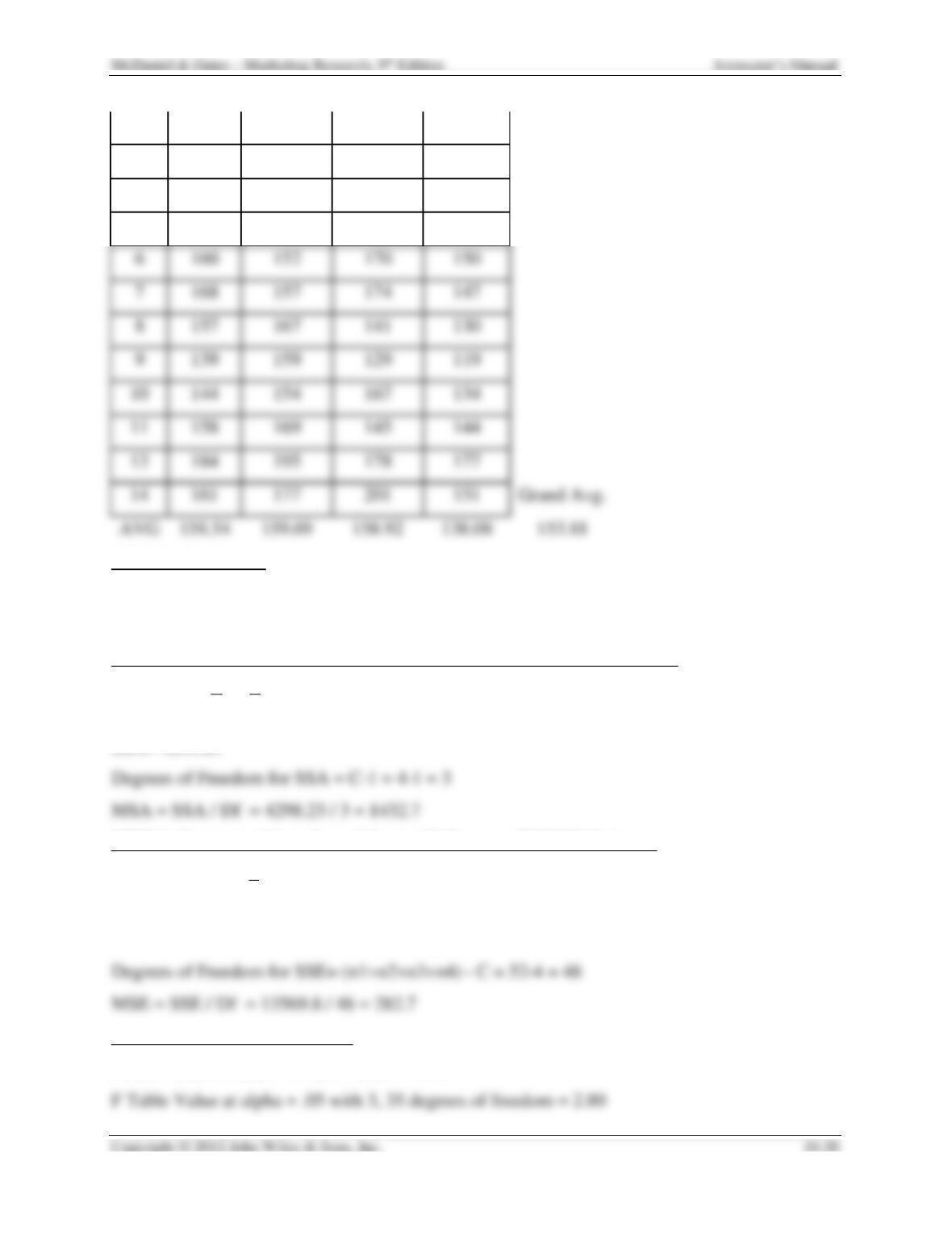
Day
Caesar
Ranch-
Style
Green
Goddess
Russian
1
155
143
149
135
Instructor’s Manual
2
157
146
152
136
3
151
141
146
131
4
146
136
141
126
5
181
180
173
115
6
160
152
170
150
7
168
157
174
147
8
157
167
141
130
9
139
159
129
119
144
154
167
134
158
169
145
144
184
195
178
177
161
177
201
151
STEP 1: Hypotheses
H0: M1M2M3 M4; mean request for the four salad dressings are equal.
Ha: The variability in group means is greater than would be expected because of sampling error.
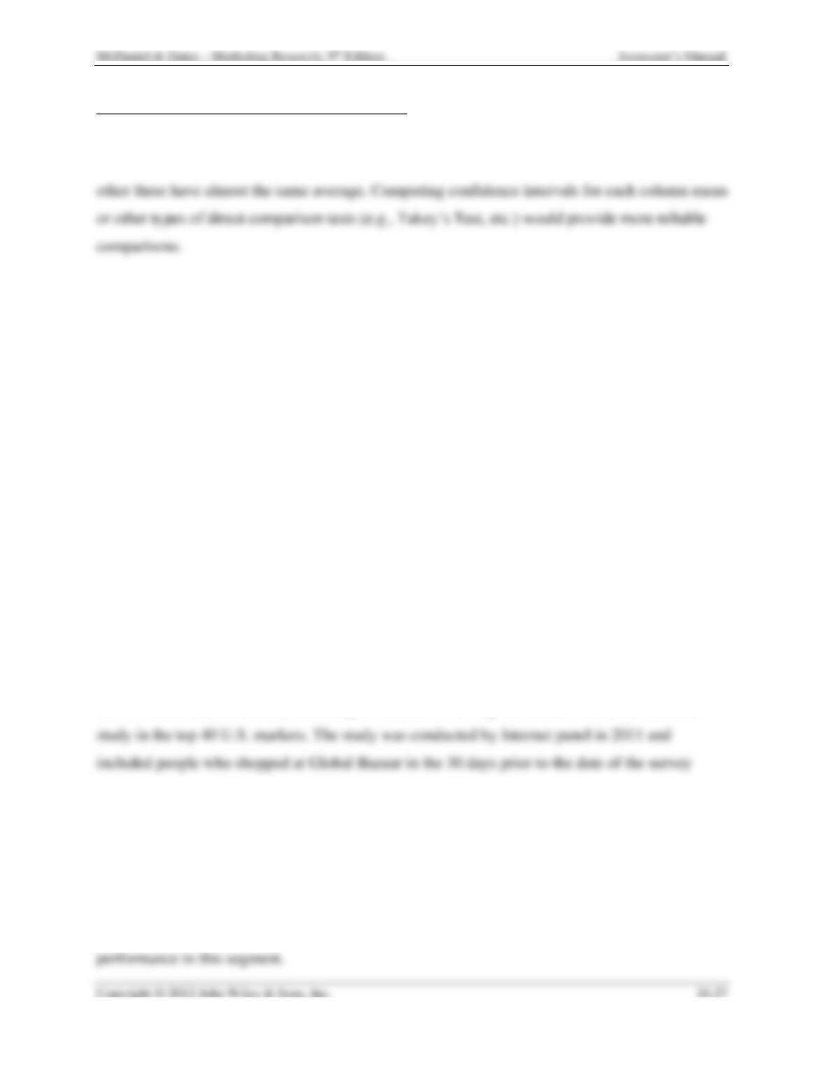
STEP 2: Determine Mean Sum of Square Differences BETWEEN Columns
SSA =njX j−X
t
( )2
j=1
C
=13 158.5 −153.8
( )2+159.7 −153.8
( )2+158.9 −153.8
( )2+138.1−153.8
( )2
SSA= 4298.23
STEP 3: Determine Mean Sum of Square Differences WITHIN Columns
SSE =
j=1
C
Xij −X j
( )2
i=1
nj
SSE=2075.2 +3574.8+4792.9+3126.9 = 13569.8
STEP 4: Calculate the F statistic
F calc = MSA / MSE = 1432.7 / 282.7 = 5.07
Instructor’s Manual
STEP 5: Compare Results and State Conclusion
Fcalc > Ftable. Hence, there is at least one mean that is statistically different from the rest.
Looking at the results, it would appear that Russian Dressing has the least appeal whereas the
WORKING THE NET
1. Calculating the p value and performing a Z or t test are much easier when done by
computers.
For a p value calculator, usable without fee, visit: www.graphpad.
com/quickcalcs/PValue1.cfm
For a Z test calculator, also free to use, visit: www. changbioscience. com/stat/ztest.html
For a t test online calculator, available also with no charge, visit:
www.graphpad.com/quickcalcs/ttest1.cfm
2. Educators at Tufts University offer a helpful tutorial on reading the output from a one-
way analysis of variance, an ANOVA table. Study this at:
http://www.JerryDallal.com/LHSP/aov1out.htm
REAL-LIFE RESEARCH
Case 16.1 – Global Bazaar (p 508-509)
Key Points:
Nala Chan is an advertising executive with Stewart Bakin Advertising. She is responsible
for the Global Bazaar account and has just finished reviewing the results of a recent customer
Questions
1. Which segment provides the largest percentage of sales?
2. In which segment does Global have the highest top of mind awareness?
3. Which two segments account for over 60 percent of sales?
4. In what segment does Global perform most poorly? Explain all the dimensions of their poor
5. Based on these results, what advice would you give to Global?
Case 16.2 – New Mexico Power (p 509)
Key Points:
• Marc Guerraz is the new marketing research director for New Mexico Power (NMP), an
investor–owned, vertically integrated electric utility involved in the generation,
transmission, distribution and energy service domains of the electricity service industry.
NMP will become part of a competitive environment in one year.
Questions
1. How could the error range be reduced without collecting more data? Would you
recommend taking this approach? Why/Why not?
2. Do you think New Mexico Power senior management would find this approach to
reducing the error range as satisfactory?
95 percent confidence level is quite high. Most business decisions do not require that degree of
3. If 500 more respondents were surveyed and 30 percent of the sample still indicated they
would switch, what would the error range become?
Instructor’s Manual
The relationship is based upon a square, if you double the sample size you reduce the error by
SPSS EXERCISE CHAPTER 16
EXERCISE #1: Analyzing Data Using Cross-tabulation Analysis
1. What % of males do not attend movies at movie theaters?
2. What % of all respondents are African American and do not attend movies at movie
theaters?
0.6 %
3. What % of respondents not attending movies at movie theaters is in the 19 – 20 age
category?
4. What classification group is least likely to attend movies at a movie theater?
5. What age category is least likely to attend movies at a movie theater?
6. Are Caucasians less likely to attend movie theaters than African Americans?
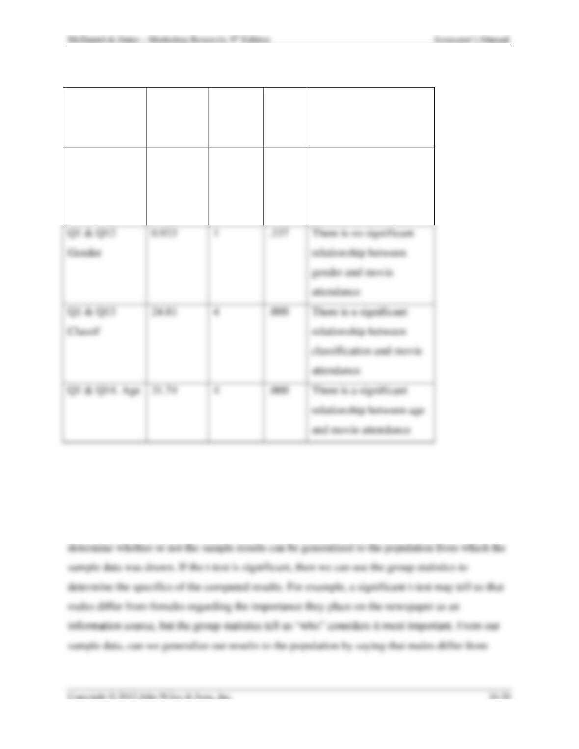
7. Evaluate the chi-square statistic in each of your crosstab tables. Construct a table to
summarize the results. For example:
Instructor’s Manual
Evaluation Table
Variables
Pearson
Chi-
Square
Degrees
of
Freedom
Asymp
sig
Explanation
Q1 & Q11
Ethnicity
4.792
3
.118
There is no significant
relationship between
ethnicity and movie
attendance
Q1 & Q14. Age
31.74
4
.000
There is a significant
and movie attendance
EXERCISE #2: t/ Z Test for Independent Samples
The result of the t-test generates a table of group statistics which is based only on the sample
data. The other output table generated by the t-test has statistical data from which we can
1. The newspaper (Q7a)? Yes. .001
2. The Internet (Q7b)? No. .204
3. Phoning in to the movie theater for information (Q7c)? Yes. .001
4. The television (Q7d)? No. .491
5. Friends or family (Q7e)? No. .333
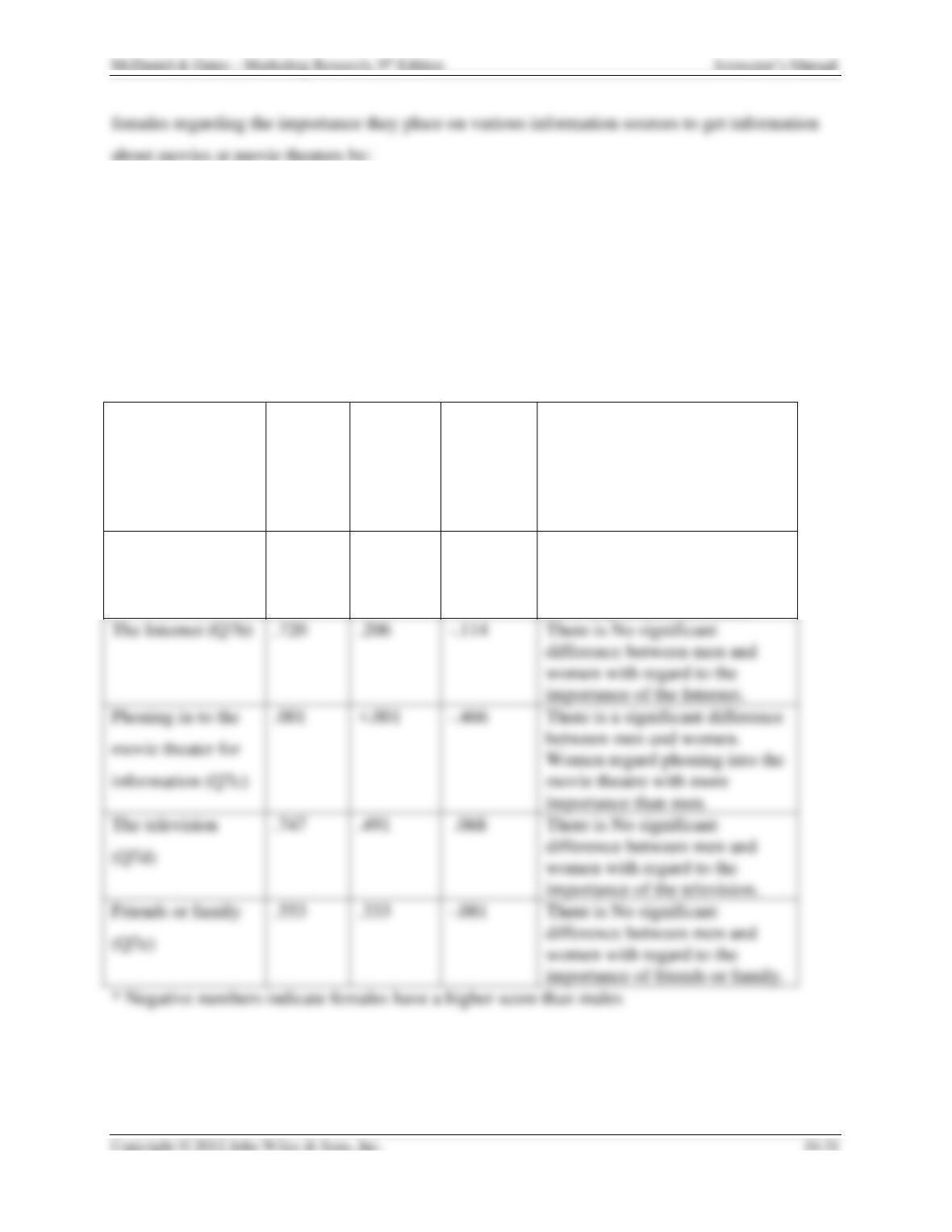
Interpretation Table
Variables
Variance
Prob
of Sig
Diff
Means
Prob
of Sig
Diff
Difference
in Means*
Interpretation
The newspaper
(Q7a)
.001
<.001
-.369
There is a significant difference
between men and women.
Women regard newspapers with
more importance than men.
information (Q7c)
between men and women.
Women regard phoning into the
movie theatre with more
importance than men.
The television
(Q7d)
.747
.491
.068
There is No significant
difference between men and
women with regard to the
importance of the television.
Friends or family
(Q7e)
.553
.333
-.081
There is No significant
difference between men and
women with regard to the
importance of friends or family.
EXERCISE #3: ANOVA Test for Independent Samples
Invoke the analyze/compare means/One-Way ANOVA sequence to invoke the ANOVA test to
complete this exercise. This exercise compares the responses of freshmen, sophomores, juniors,
seniors, and graduate students to test for significant differences in the importance placed on
several movie theater items. For the ANOVA test, SPSS calls the variable in which means are
being computed the independent variable and the variable in which we are grouping responses
1. Video arcade at the movie theater (Q5a)? No. .548
2. Soft drinks and food items (Q5b)? No. .117
3. Plentiful restrooms (Q5c)? Yes .026
4. Comfortable chairs (Q5d)? No. .819
9. Clean restrooms (Q5i)? No. .885
10. Using only descriptive statistics, which classification group (Q13) places the least amount of
importance on clean restrooms (Q5i)? Graduate students, 3.47.
11. Using only the descriptive statistics, which classification group (Q13) places the greatest
amount of importance on quality of sound system (Q5i)? Juniors, 3.63.
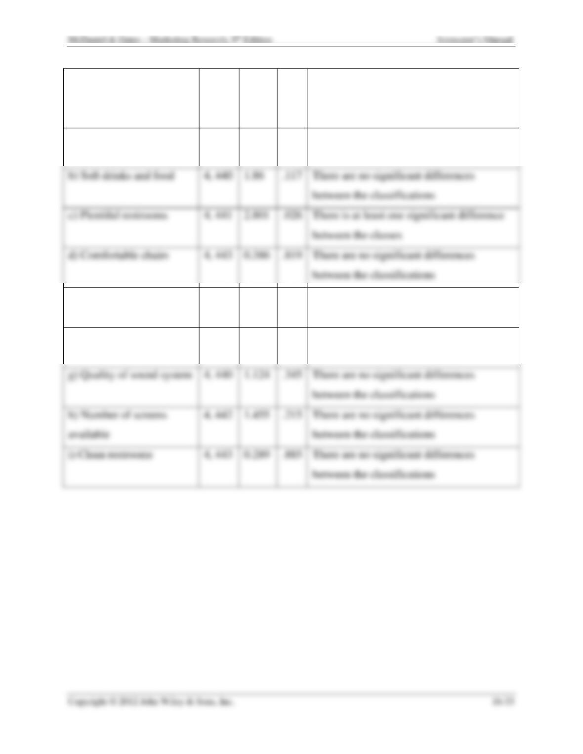
Instructor’s Manual
How important is the
following when choosing a
movie theatre…
DF
Fcalc
Sig
Interpretation
a) Video Arcade at the
Movie Theatre
4, 442
0.766
.548
There are no significant differences
between the classifications
b) Soft drinks and food
4, 440
1.86
.117
There are no significant differences
between the classifications
c) Plentiful restrooms
4, 441
2.801
.026
There is at least one significant difference
between the classes
d) Comfortable chairs
4, 443
0.386
.819
There are no significant differences
between the classifications
e) Auditorium type seating
4, 443
0.223
.925
There are no significant differences
between the classifications
f) Size of screen(s)
4, 441
1.153
.331
There are no significant differences
between the classifications
i) Clean restrooms
4, 443
0.289
.885
There are no significant differences
between the classifications