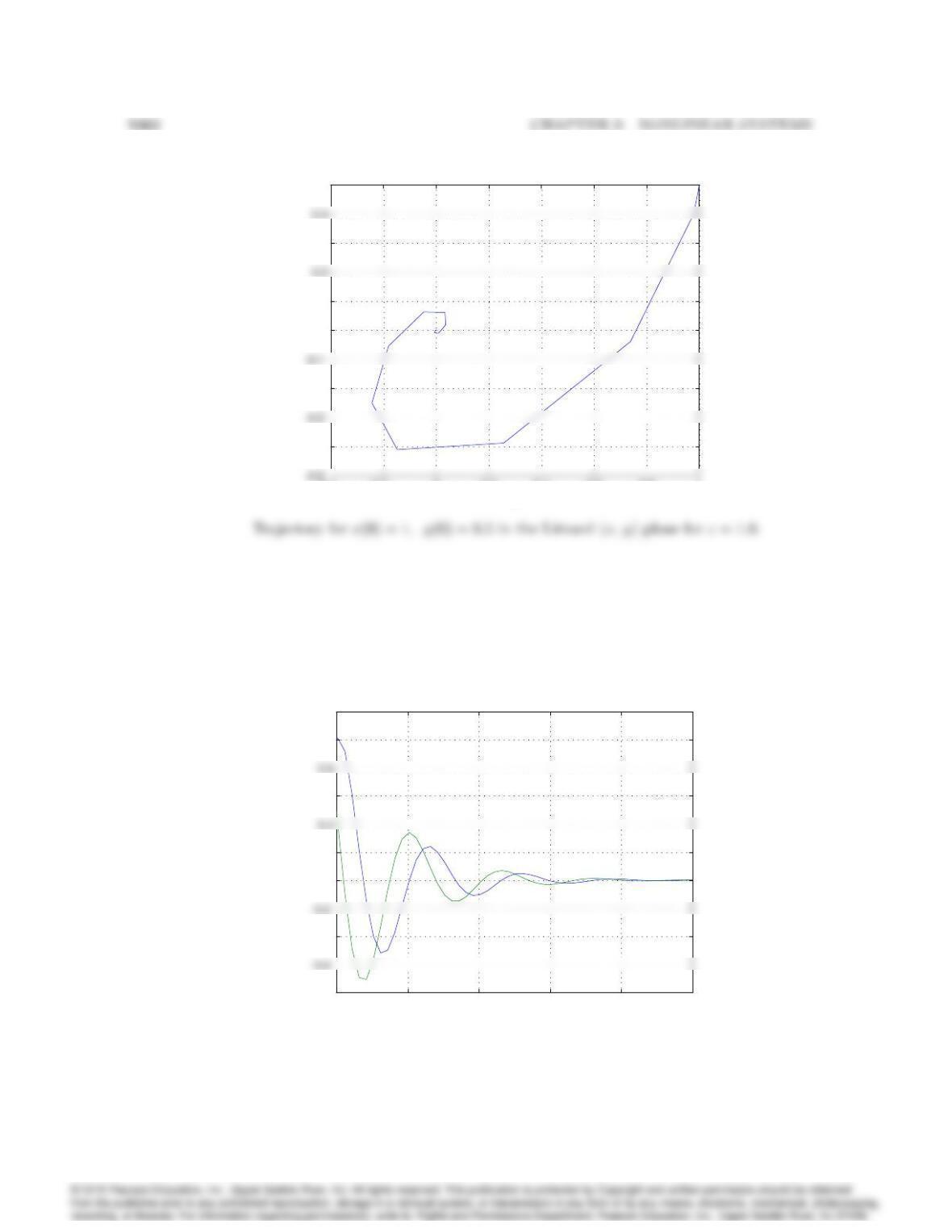
–0.4 –0.2 00.2 0.4 0.6 0.8 1
–0.4
–0.2
0
0.1
0.3
0.5
y
x
The corresponding time domain responses are shown in the attached figures.
0 5 10 15 20 25
–0.8
–0.4
0
0.2
0.6
1
1.2
Time (sec)
x,y
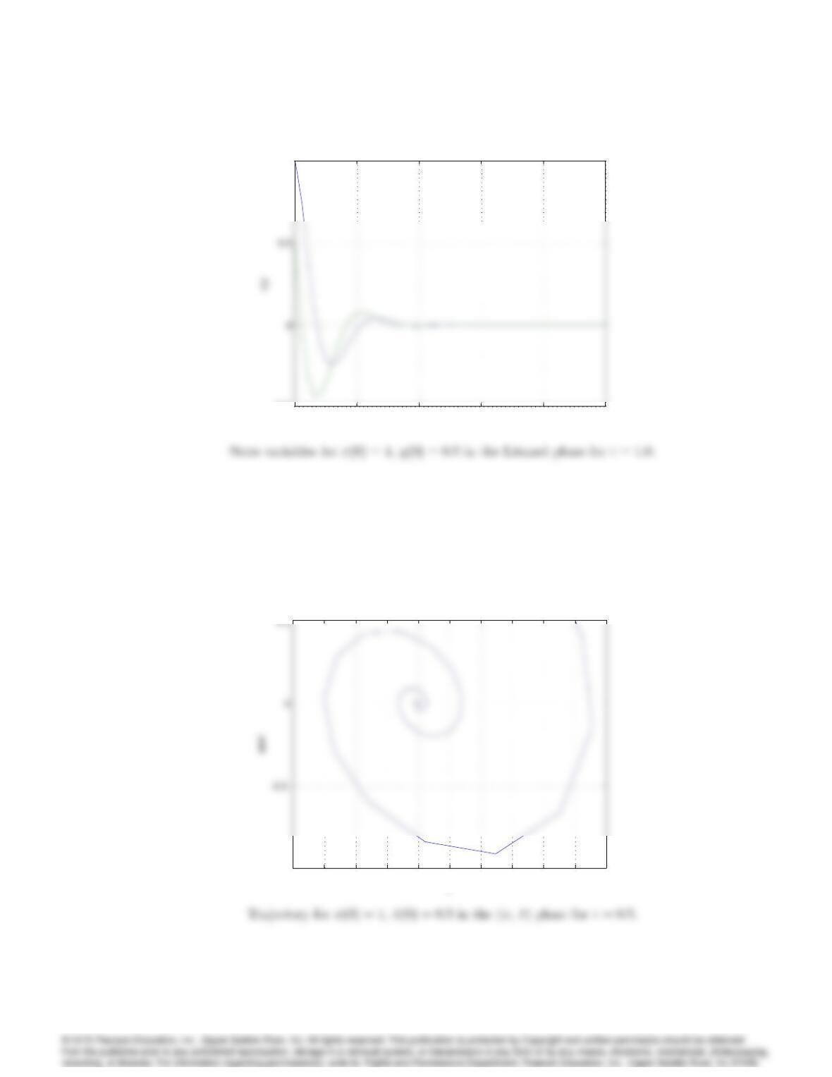
State variables for x(0) = 1,y(0) = 0:5in the Liénard (x,y) plane for “= 0:5.
9061
0 5 10 15 20 25
–0.5
1
Time (sec)
–0.8 -0.6 –0.4 –0.2 00.2 0.4 0.6 0.8 1
-1
x
–0.4 –0.2 00.2 0.4 0.6 0.8 11.2
-1
0.5
x
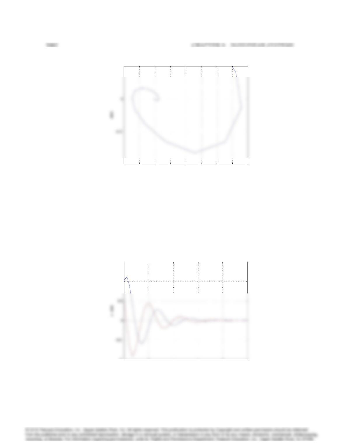
Trajectory for x(0) = 1,_x(0) = 0:5in the (x,_x) plane for “= 1:0.
0 5 10 15 20 25
-1
1
1.5
Time (sec)
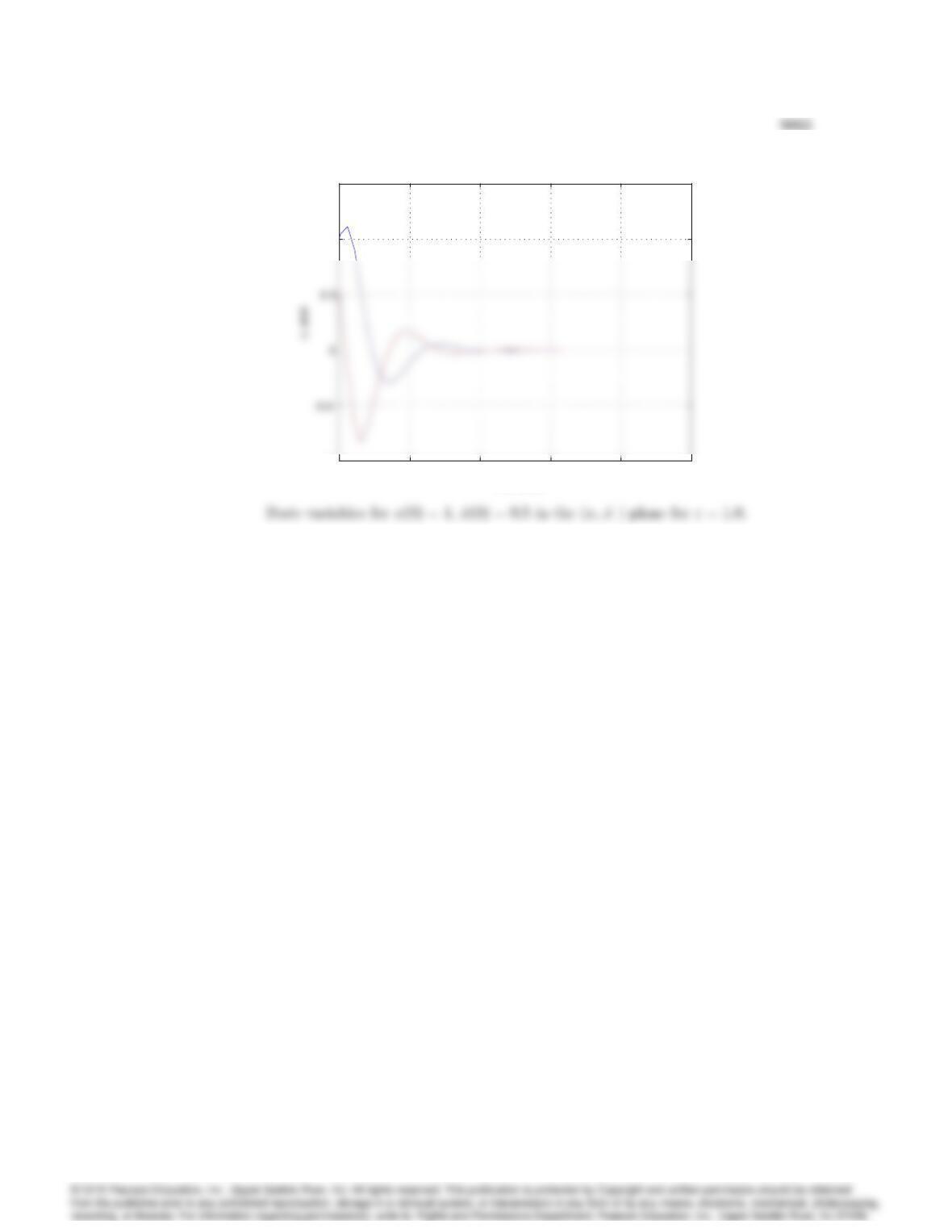
State variables for x(0) = 1,_x(0) = 0:5in the (x,_x) plane for “= 0:5.
0 5 10 15 20 25
-1
1
1.5
Time (sec)
34. Du¢ng’s equation: Consider the system described by the nonlinear differential equation
•x+k_x+“x3=u
where u=Acos(t). This equation represents the model of a hard spring where kis the spring
constant and if ” > 0, the spring gets stiffer as the displacement increases. Let k= 0:05,= 1,
and A= 7:5.
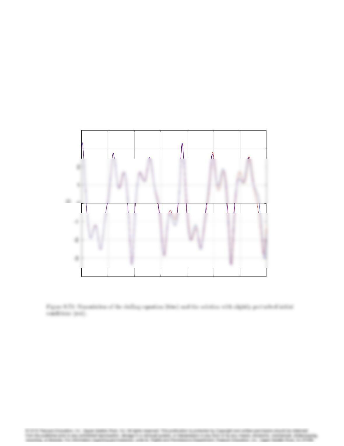
(a) Build a simulation of the system in SIMULINK. Show that the system response can be very
sensitive to slight perturbations on the initial conditions x(0),_x(0) (the system is said to
be chaotic). Simulate the response of the system with x(0) = 3 and _x(0) = 4 for t= 30 sec.
Repeat the simulation for slightly perturbed initial conditions x(0) = 3:01 and _x(0) = 4:01.
Compare the two results.
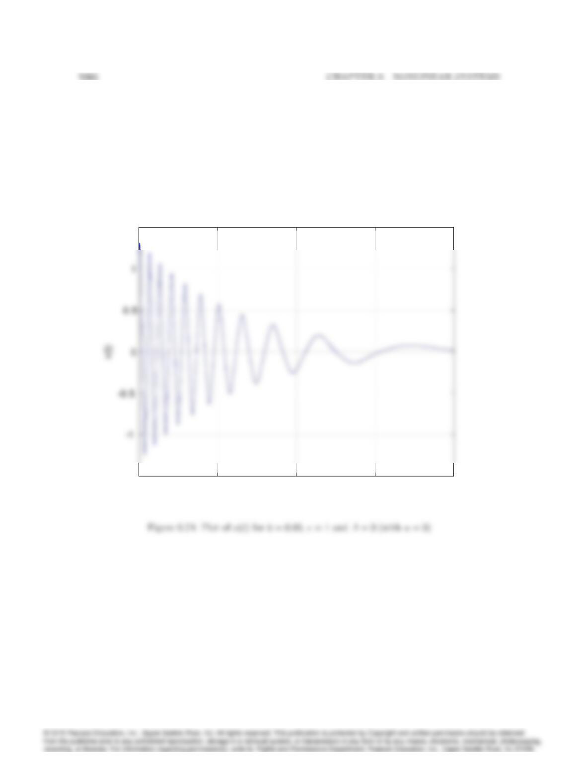
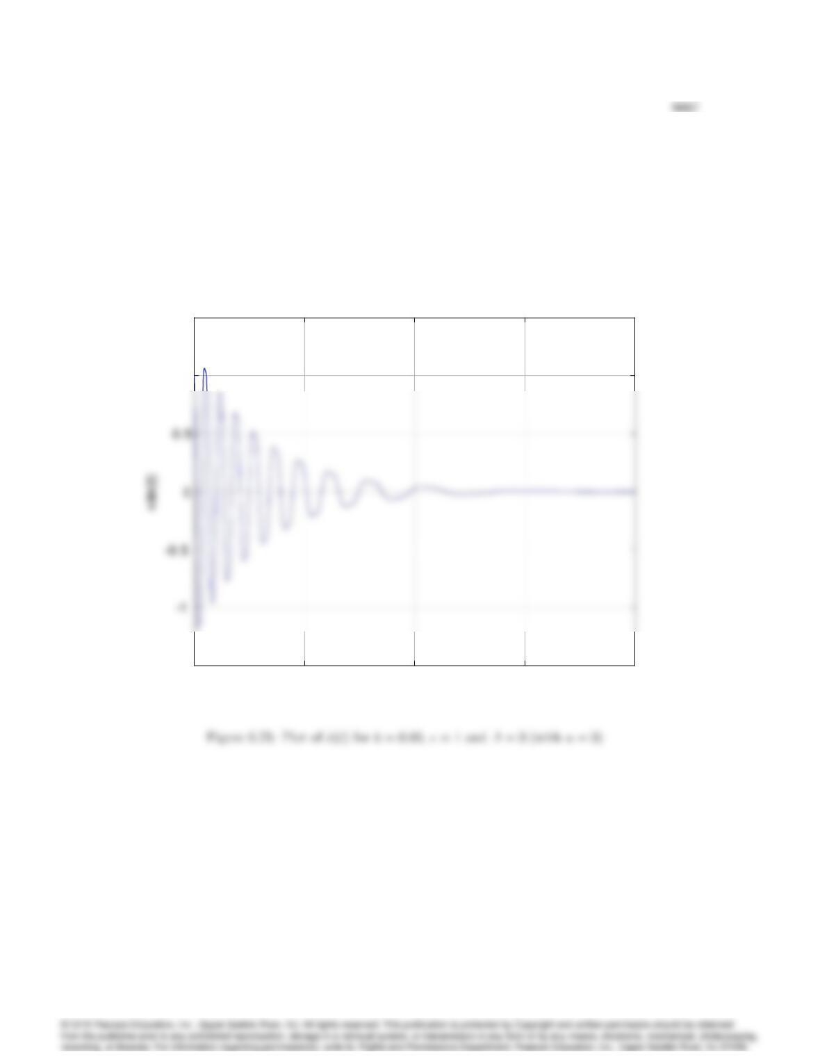
(b) Consider the unforced Du¢ng equation (u= 0). Plot the time response of the system for
x(0) = 1,_x(0) = 1 for t= 200 sec. Draw the phase-plane plot for the system. Show that
the origin is an equilibrium point.
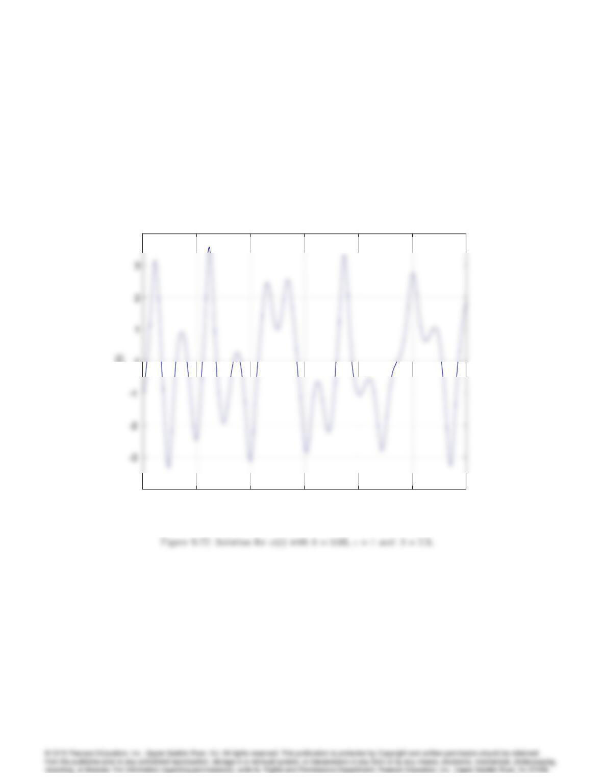
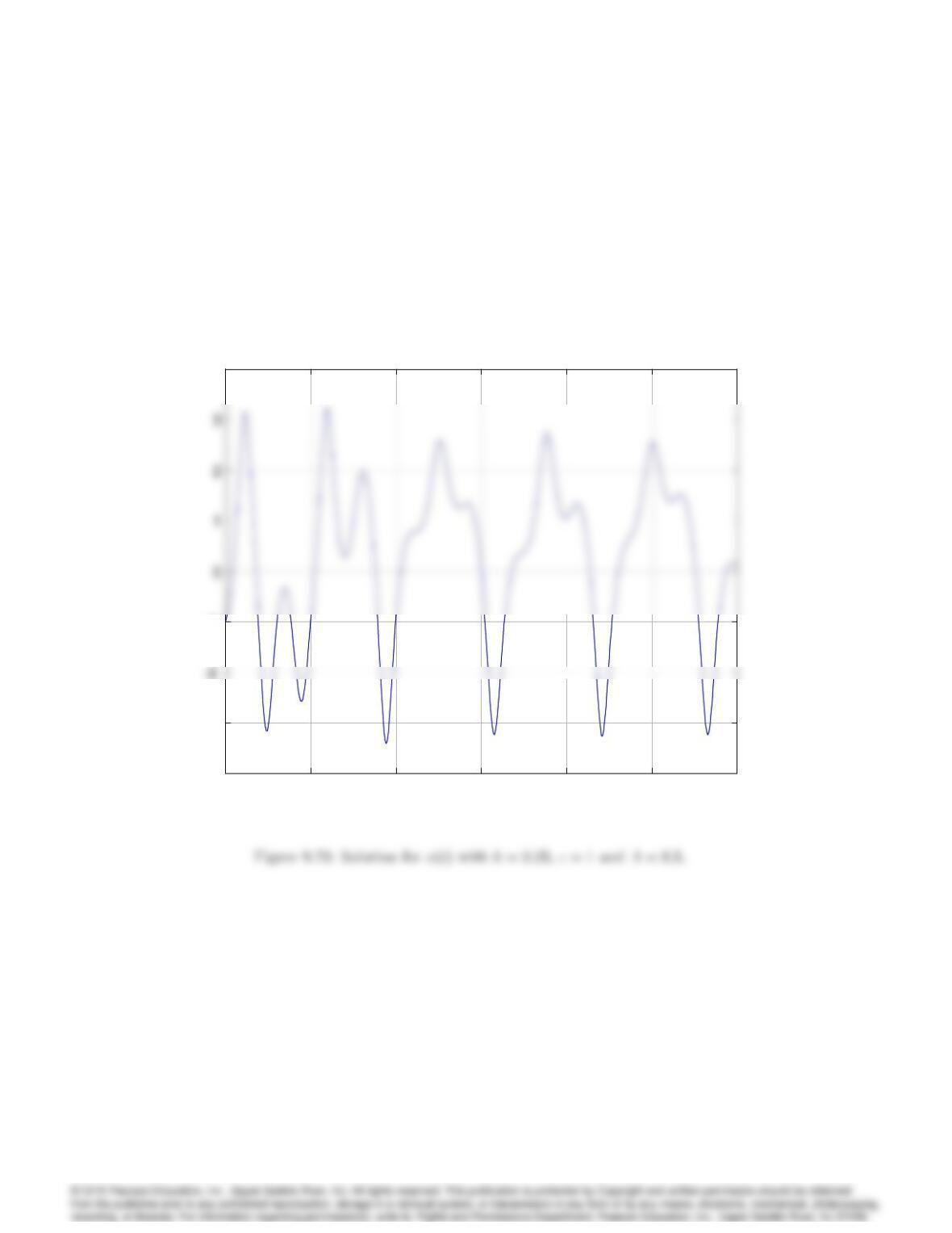
(c) Now consider the forced Du¢ng equation (u6= 0). Find the solution to the Du¢ng equation
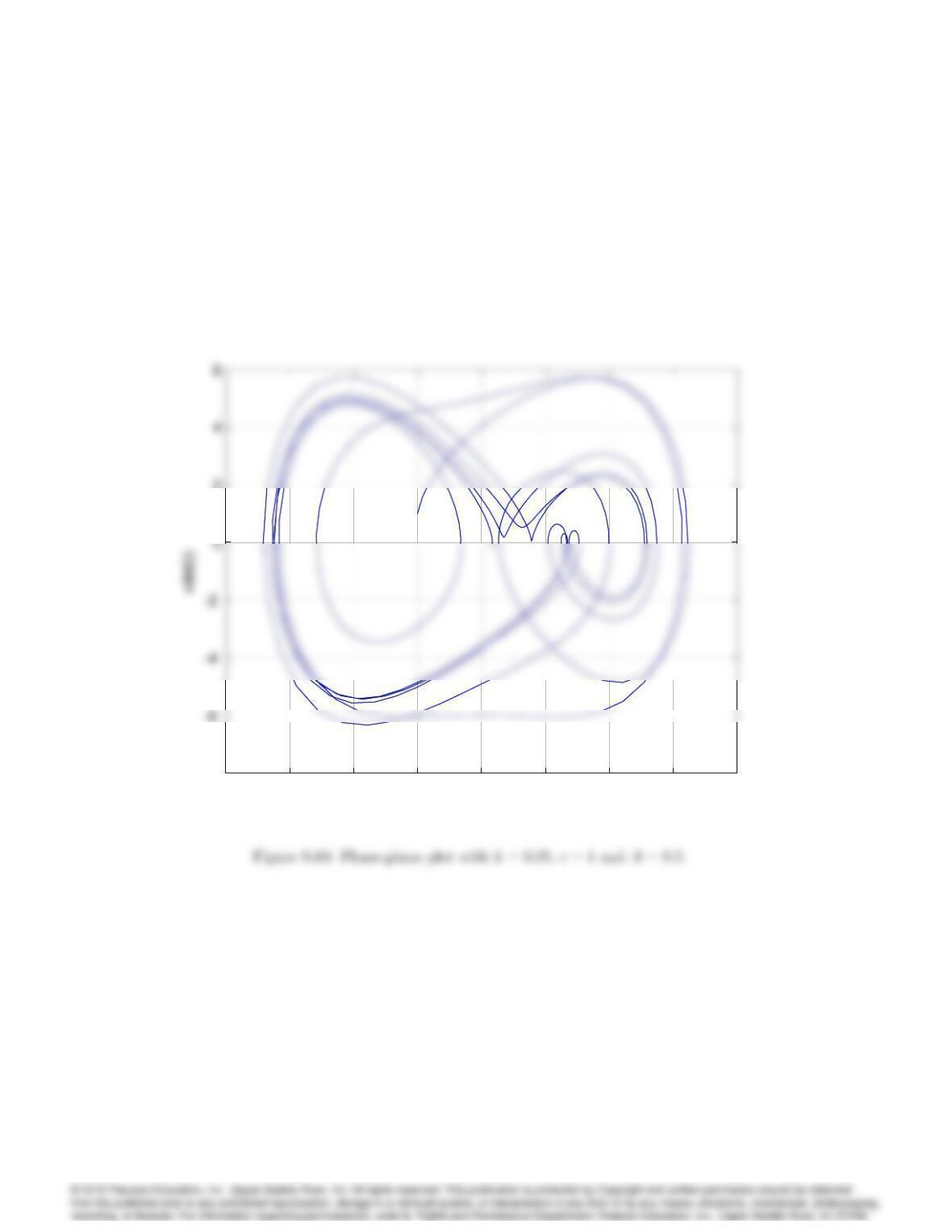
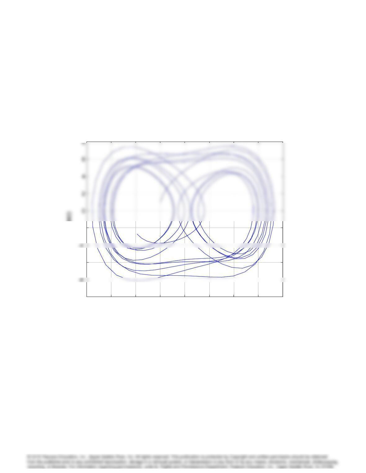
for x(0) = 1,_x(0) = 1 for t= 30 sec. Draw the phase-plane plot ( _x(t)vs. x(t)) for this
case.
(d) Repeat part (c) for k= 0:25,= 1, and A= 8:5.
(e) Repeat part (c) for k= 0:1,= 1, and A= 11.
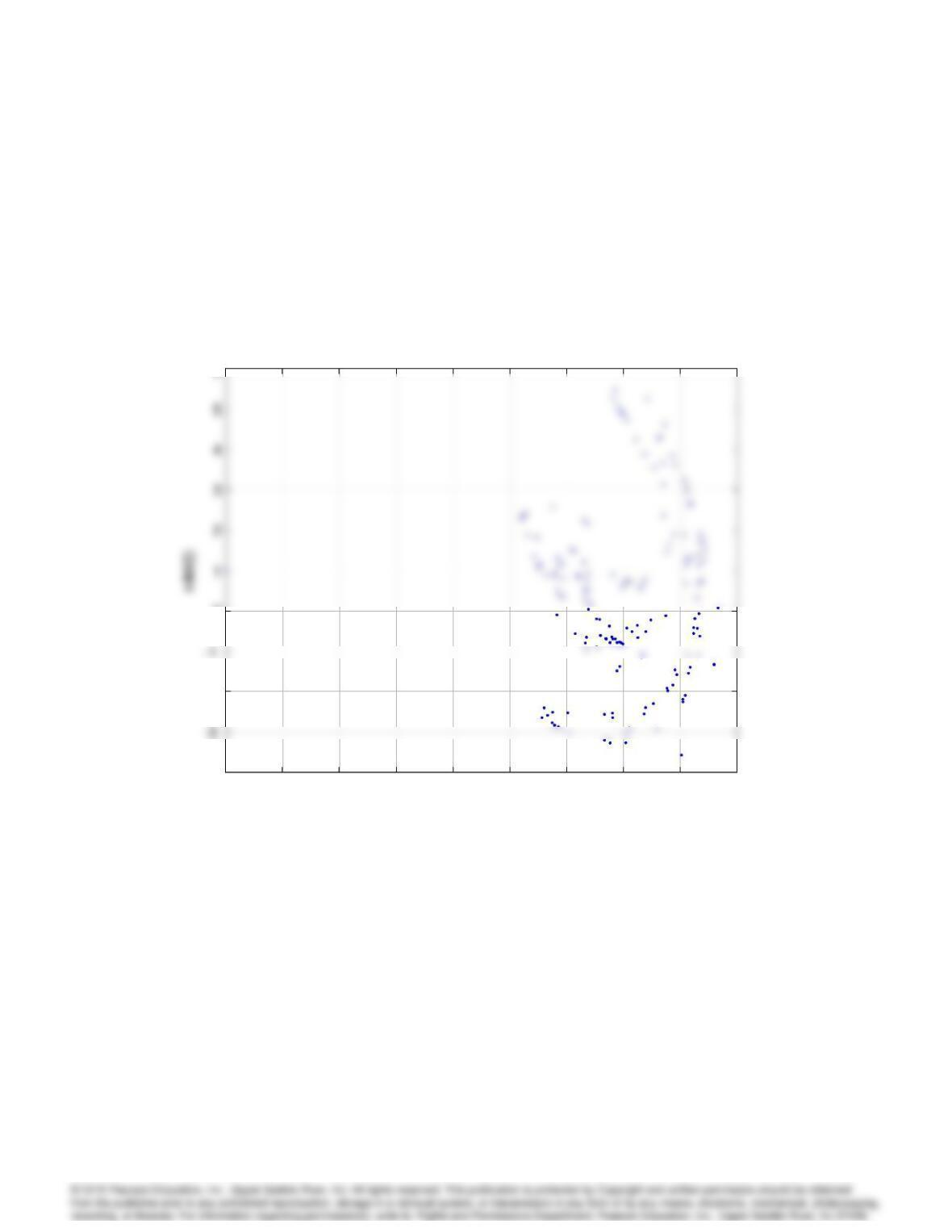
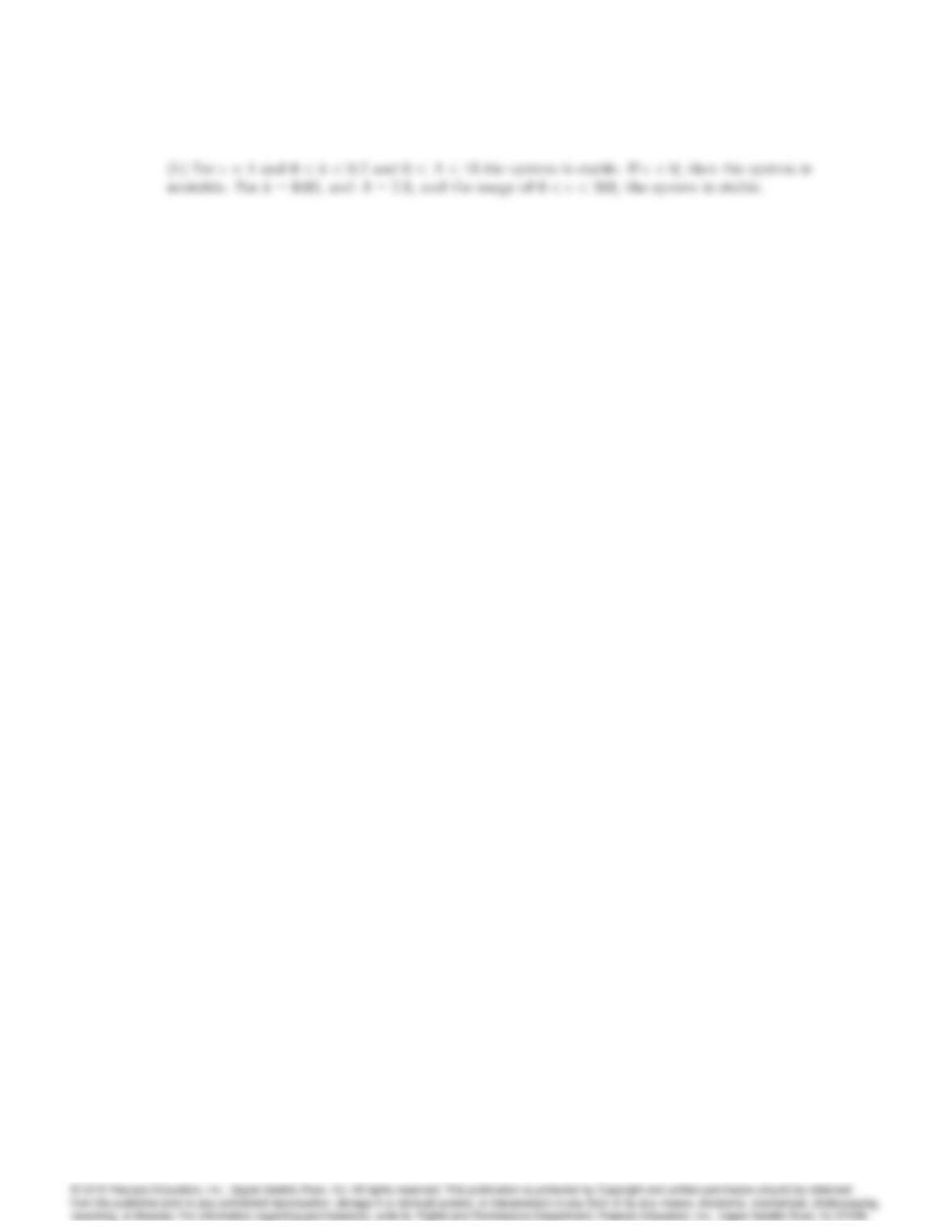
(f) We can get more insight into the system by plotting _x(tj)vs. x(tj)at several hundred
points at 2periodic observation times. In other words rather than looking at the system
continuously, we “strobe” the system and plot the behavior at strobe times only. Show that
unlike the parametric plots in parts (c)-(e), the points fall on a well-structured plot referred
to as a Poincaré section (also called a strange attractor). Plot the Poincaré sections for
parts (c)-(e). Simulate the system using the initial conditions x(0) = 1and _x(0) = 1 for
t= 10;000 sec in order to plot the Poincaré sections.
9064 CHAPTER 9. NONLINEAR SYSTEMS
Figure 9.72: Simulation of the Du¢ng equation.
(g) What can you conclude about the nature of the solution of the Du¢ng equation from the
results of the previous parts?
(h) Characterize the system behavior in terms of the ranges of the system parameters k,, and
A.
Solution:
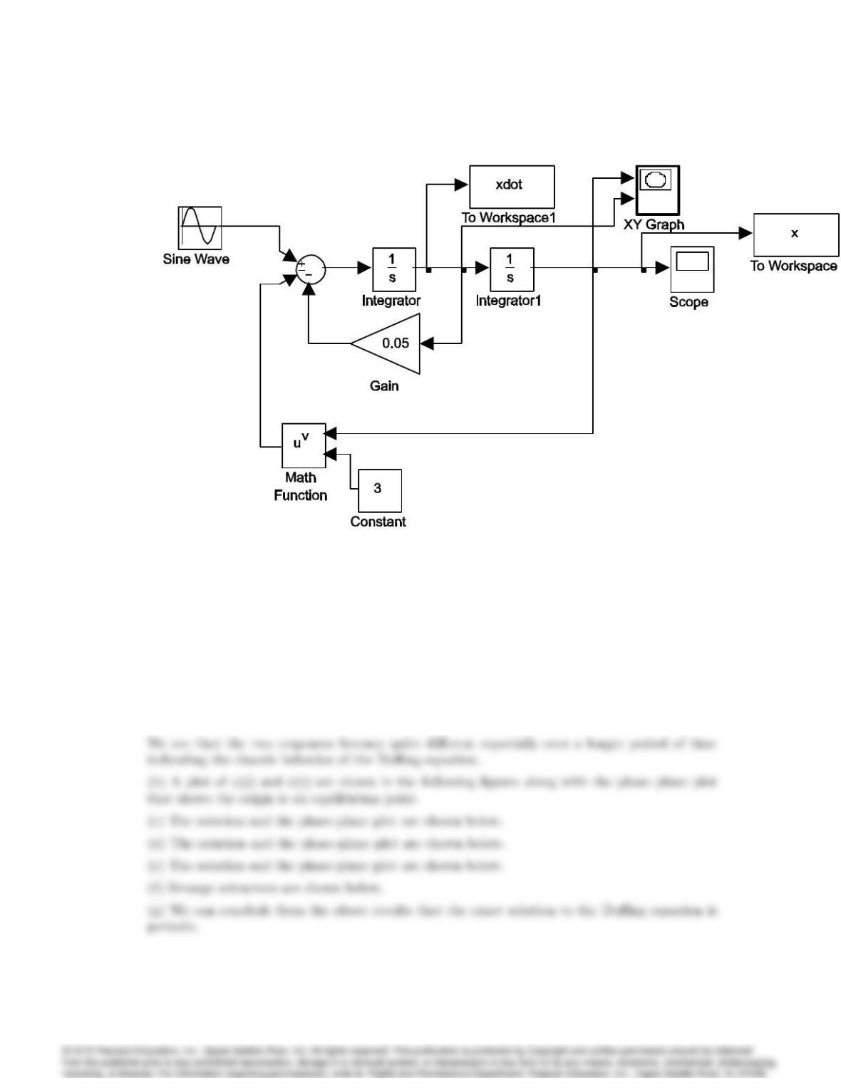
(a) The SIMULINK implementation of the system is shown in the following figure.
9065
0 5 10 15 20 25 30 35
-4
0
3
4
x(t)
Time (sec)
0 5 10 15 20 25 30 35
-4
0
3
4
x(t)
Time (sec)
050 100 150 200
–1.5
1.5
Time (sec)
050 100 150 200
–1.5
1.5
Time (sec)
050 100 150 200
–1.5
1
1.5
Time (sec)
050 100 150 200
–1.5
1
1.5
Time (sec)
–1.5 -1 –0.5 00.5 11.5
–1.5
1.5
x(t)
–1.5 -1 –0.5 00.5 11.5
–1.5
1.5
x(t)
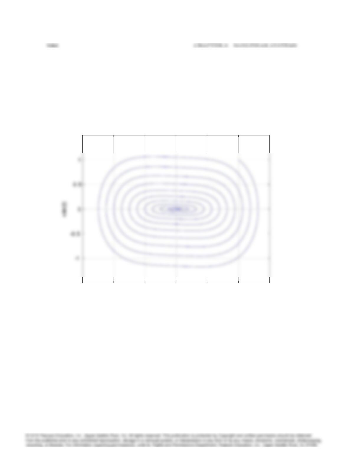
Figure 9.76: Phase plane plot for k= 0:05,= 1 and A= 0 (with u= 0)
9069
0 5 10 15 20 25 30
-4
0
4
Time (sec)
x(t)
0 5 10 15 20 25 30
-4
0
4
Time (sec)
x(t)
9070 CHAPTER 9. NONLINEAR SYSTEMS
-4 -3 -2 -1 0 1 2 3 4
-2
x(t)
-4 -3 -2 -1 0 1 2 3 4
-2
x(t)
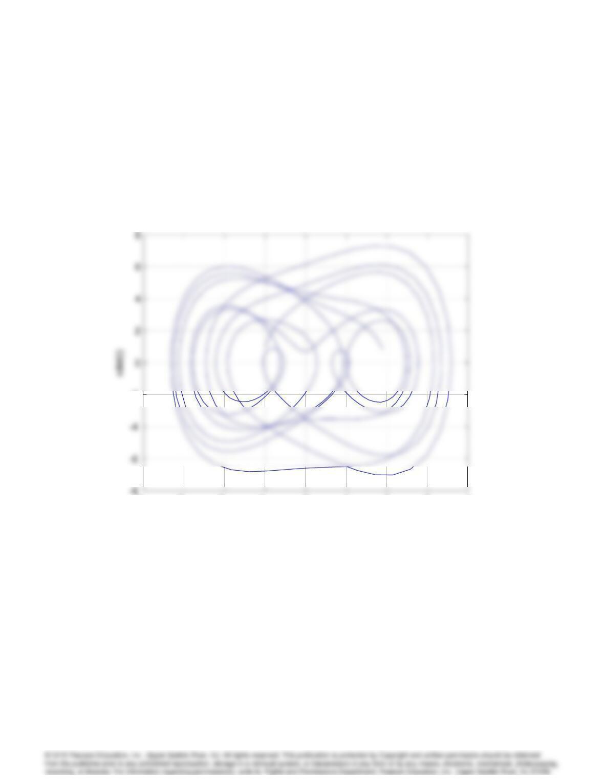
Figure 9.78: Phase-plane plot for k= 0:05,= 1 and A= 7:5.
9071
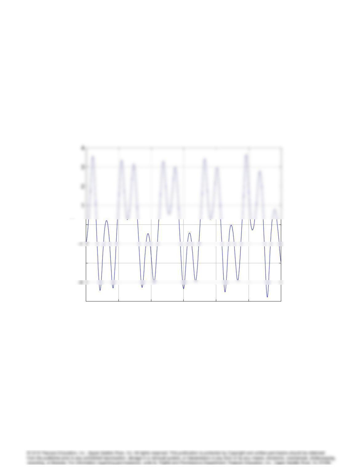
0 5 10 15 20 25 30
-4
-3
-1
4
x(t)
0 5 10 15 20 25 30
-4
-3
-1
4
x(t)
9072 CHAPTER 9. NONLINEAR SYSTEMS
-4 -3 -2 -1 0 1 2 3 4
-8
2
x(t)
-4 -3 -2 -1 0 1 2 3 4
-8
2
x(t)
9073
0 5 10 15 20 25 30
-4
-2
0
Time (sec)
x(t)
0 5 10 15 20 25 30
-4
-2
0
Time (sec)
x(t)
9074 CHAPTER 9. NONLINEAR SYSTEMS
-4 -3 -2 -1 0 1 2 3 4
–10
-6
-2
x(t)
xdot(t)
-4 -3 -2 -1 0 1 2 3 4
–10
-6
-2
x(t)
xdot(t)
Figure 9.81: Phase-plane plot with k= 0:1,= 1 and A= 12.
9075
-1 –0.5 00.5 11.5 22.5 33.5
-4
-2
0
6
x(t)
-1 –0.5 00.5 11.5 22.5 33.5
-4
-2
0
6
x(t)
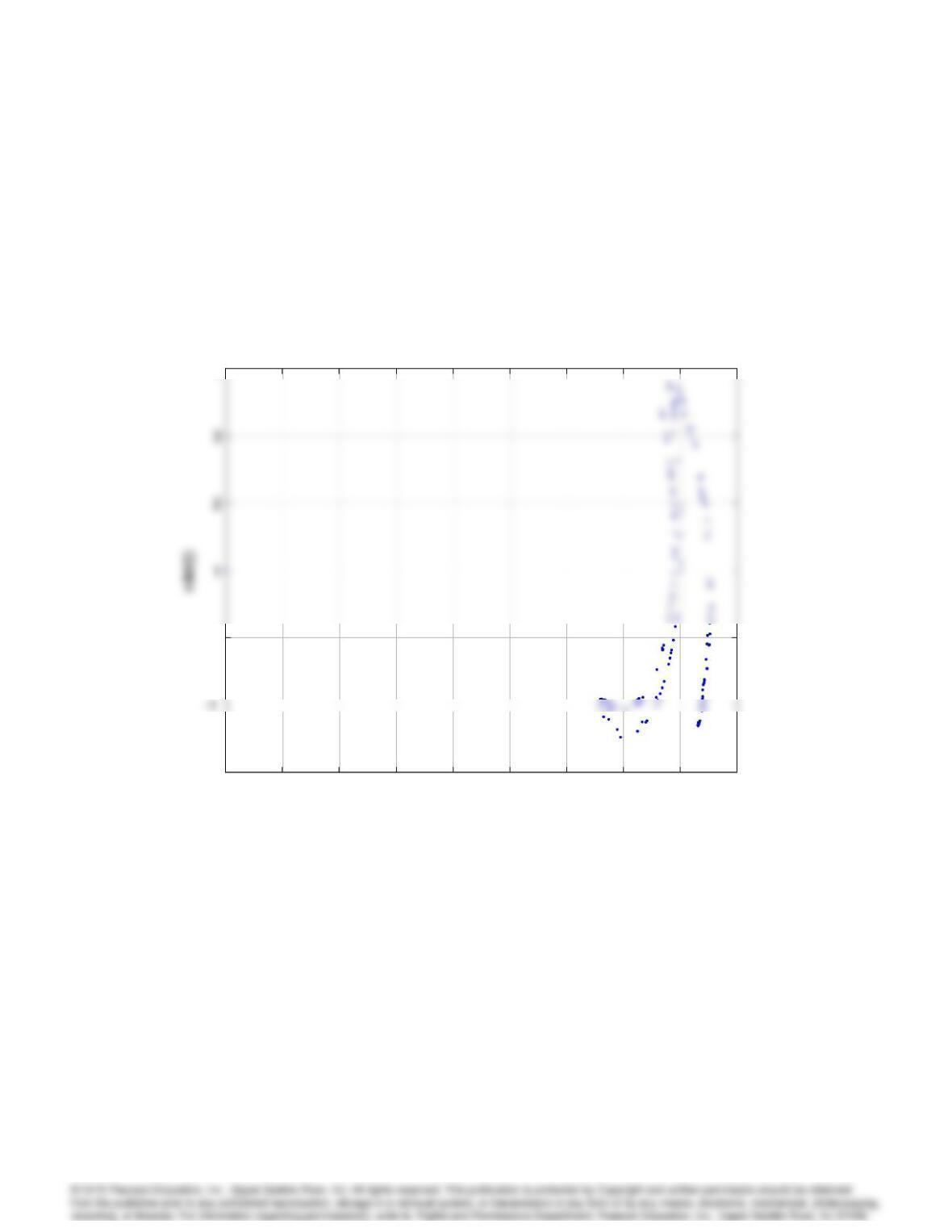
Figure 9.82: Poincaré section ( _x(tj)vs x(tj)) for k= 0:05,= 1, and A= 7:5.
9076 CHAPTER 9. NONLINEAR SYSTEMS
-1 –0.5 00.5 11.5 22.5 33.5
-2
0
4
x(t)
-1 –0.5 00.5 11.5 22.5 33.5
-2
0
4
x(t)
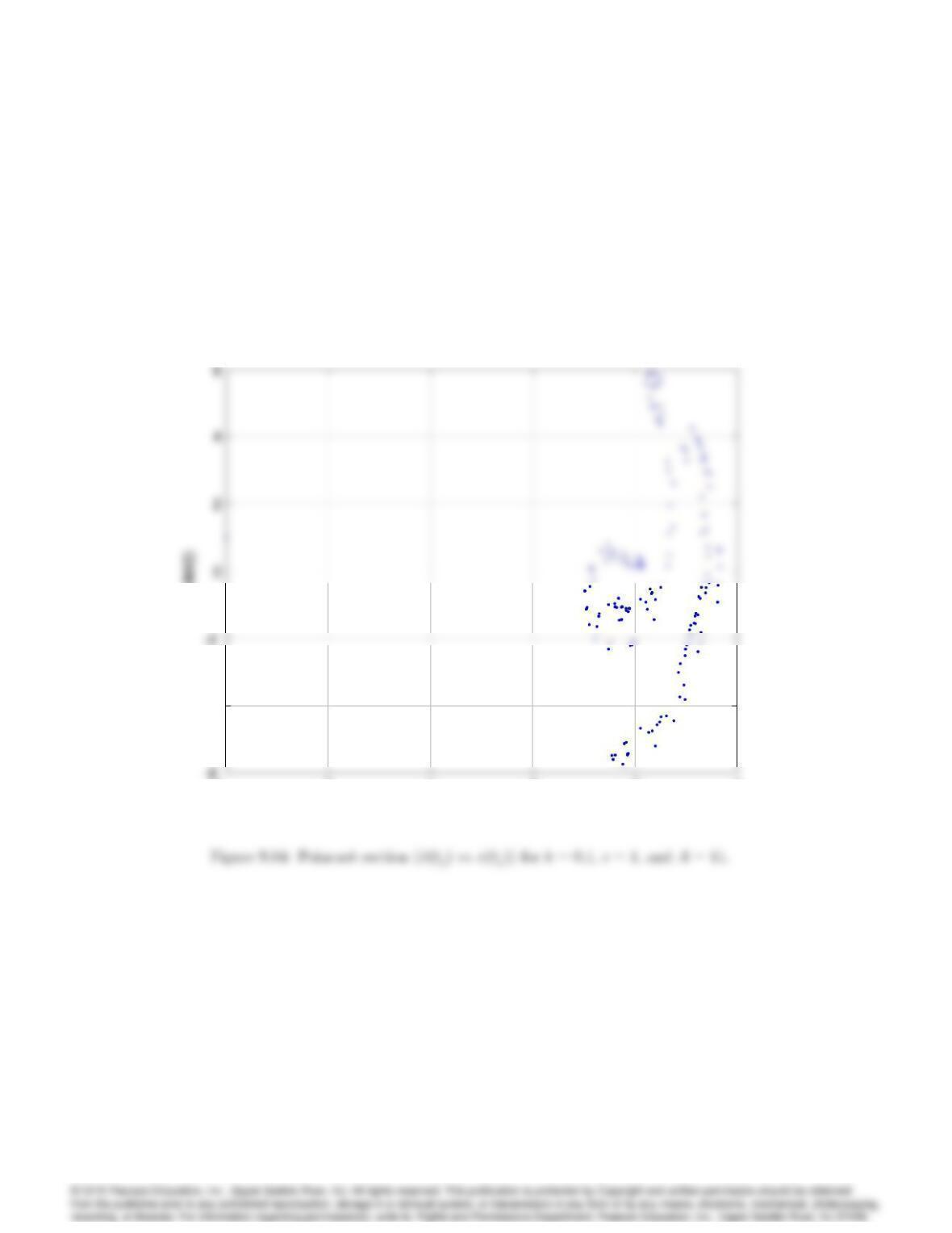
Figure 9.83: Poincaré section ( _x(tj)vs x(tj)) for k= 0:25,= 1, and A= 8:5.
9077
-1 0 1 2 3 4
-4
x(t)
xdot(t)
-1 0 1 2 3 4
-4
x(t)
xdot(t)
9078 CHAPTER 9. NONLINEAR SYSTEMS