
Solutions Manual: Chapter 9
7th Edition
Feedback Control of Dynamic
Systems
Gene F. Franklin
J. David Powell
Abbas Emami-Naeini .
Assisted by:
H.K. Aghajan
H. Al-Rahmani
P. Coulot
P. Dankoski
S. Everett
R. Fuller
T. Iwata
V. Jones
F. Safai
L. Kobayashi
H-T. Lee
E. Thuriyasena
M. Matsuoka
J.K. Lee
1
h t
on in t
Problems and Solutions for Section . : Analysis y Lineari a–
tion
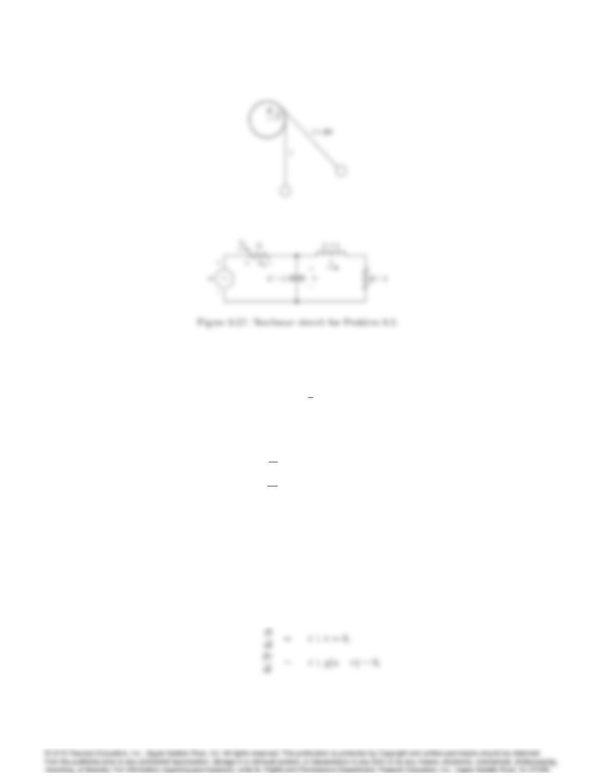
1. Figure shows a le endulum system in which a cord is wr ed around a ed cylinder.
The motion of the system that results is described by the erential e uation
(l+R)•
+gsin +R_
2= 0;
where
l= length of the cord in the vertical (down) position;
R= radius of the cylinder:
rite the state-variable for this system.
Lineari e the e uation around the oint = 0 and show that for small values of the
system on reduces to an e uation for a end that
•
+ (g=l)= 0:
This is a second order non-linear di erential on in . Let x=_
T.
For small values of .
9002 CHAPTER 9. NONLINEAR SYSTEMS
Figure 9.56: Motion of cord wrapped around a fixed cylinder
(a)
l•
+g = 0
•
+g
l= 0
2. The circuit shown in Fig. 9.57 has a nonlinear conductance Gsuch that iG=g(vG) = vG(vG
1)(vG4). The state differential equations are
di
dt =i+v;
dv
dt =i+g(uv);
where iand vare the state variables and uis the input.
(a) One equilibrium state occurs when u= 1 yielding i1=v1= 0. Find the other two pairs of
vand ithat will produce equilibrium.
(b) Find the linearized model of the system about the equilibrium point u= 1,i=v1= 0.
(c) Find the linearized models about the other two equilibrium points.
Solution:
(a) Equilibrium:
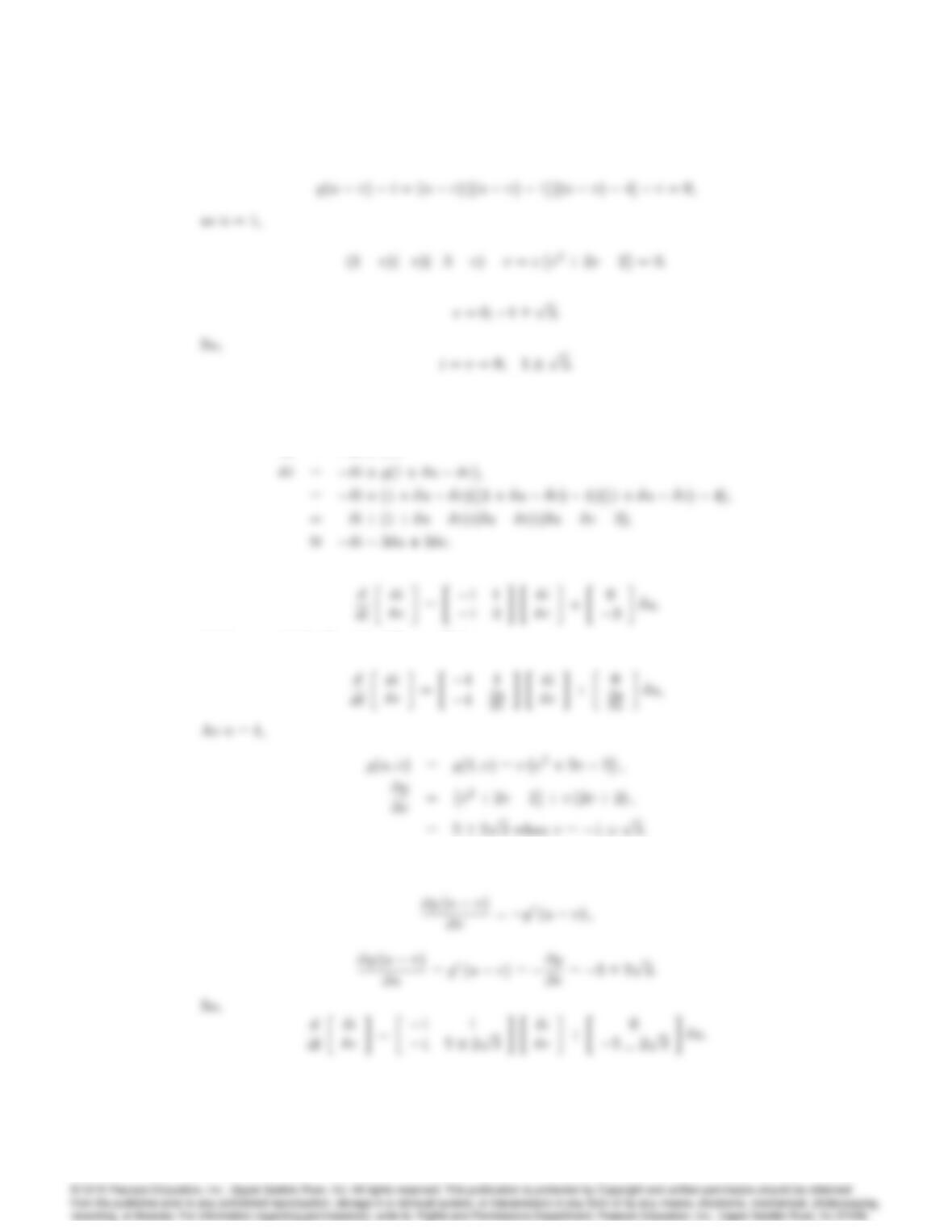
9003
(b) Let’s replace u,v, and iby 1 + u,v, and i.
_
i=i +v;
(c) In general the linearized form will be,
Also
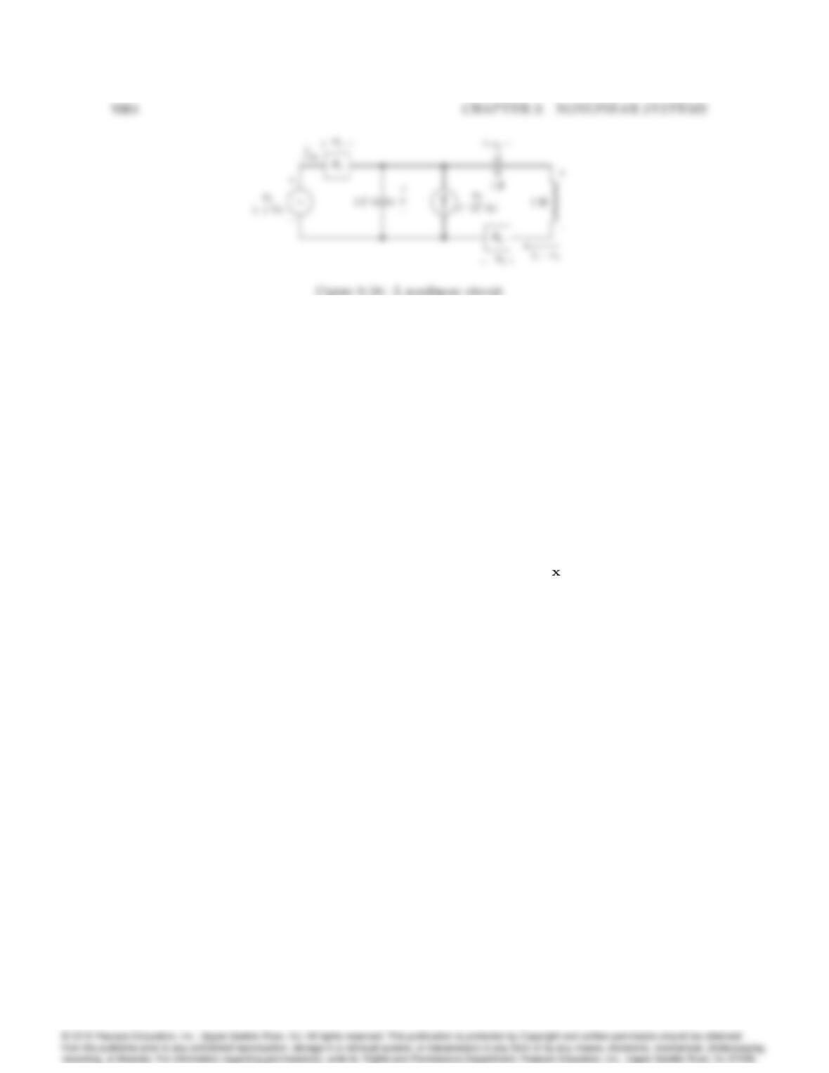
3. Consider the circuit shown in Fig. 9.58; u1and u2are voltage and current sources, respectively,
and R1and R2are nonlinear resistors with the following characteristics:
Resistor 1 : i1=G(v1) = v3
1
Resistor 2 : v2=r(i2);
where the function ris defined in Fig. 9.59.
(a) Show that the circuit equations can be written as
_x1=G(u1x1) + u2x3
_x2=x3
_x3=x1x2r(x3):
Suppose we have a constant voltage source of 1 Volt at u1and a constant current source
of 27 Amps; i.e., uo
1= 1,uo
2= 27. Find the equilibrium state o= [xo
1; xo
2; xo
3]Tfor the
circuit. For a particular input uo, an equilibrium state of the system is defined to be any
constant state vector whose elements satisfy the relation
_x1= _x2= _x3= 0:
Consequently, any system started in one of its equilibrium states will remain there indefi-
nitely until a different input is applied.
(b) Due to disturbances, the initial state (capacitance, voltages, and inductor current) is slightly
different from the equilibrium and so are the independent sources; that is,
u(t) = uo+u(t)
x(t0) = xo(t0) + x(t0):
Do a small-signal analysis of the network about the equilibrium found in (a), displaying
the equations in the form
_x1=f11 x1+f12 x2+f13 x3+g1u1+g2u2:
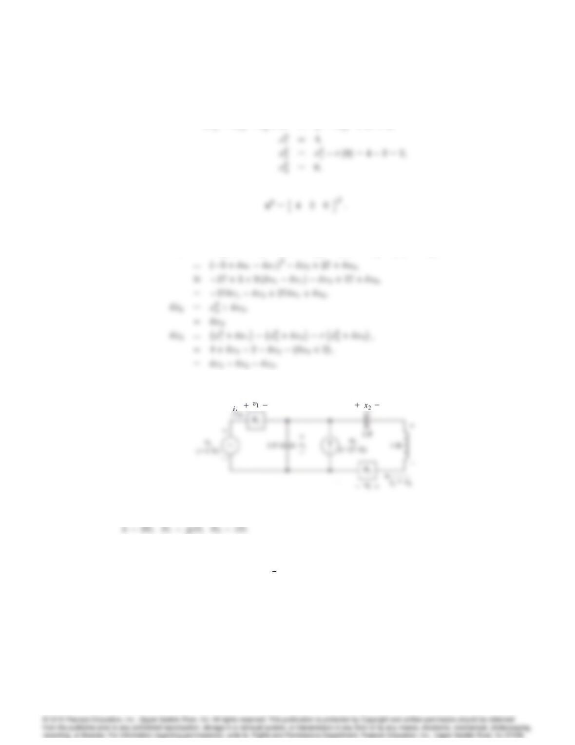
(c) Draw the circuit diagram that corresponds to the linearized model. Give the values of the
elements.
Solution:
(a)
i1=G(u1x1);
_x1=G(u1x1)x3+u2;
(b) Equilibrium state around u0
1= 1,u0
2= 27.
9006 CHAPTER 9. NONLINEAR SYSTEMS
G1x0
_x1=Gu0
1+u1x0
1+x1x0
3+x3+u0
2+u2;
(c) Circuit diagram:
Linear circuit model for Problem 9.3.
4. Consider the nonlinear system
_x=x2e1
x+ sin u x(0) = 1
a) Assume uo= 0 and solve for xo(t).
b) Find the linearized model about the nominal solution in part (a).
Solution:
9007
(a)
x;
Integrate both sides:
Zx(t)
xdx =Zt
dt;
(b)
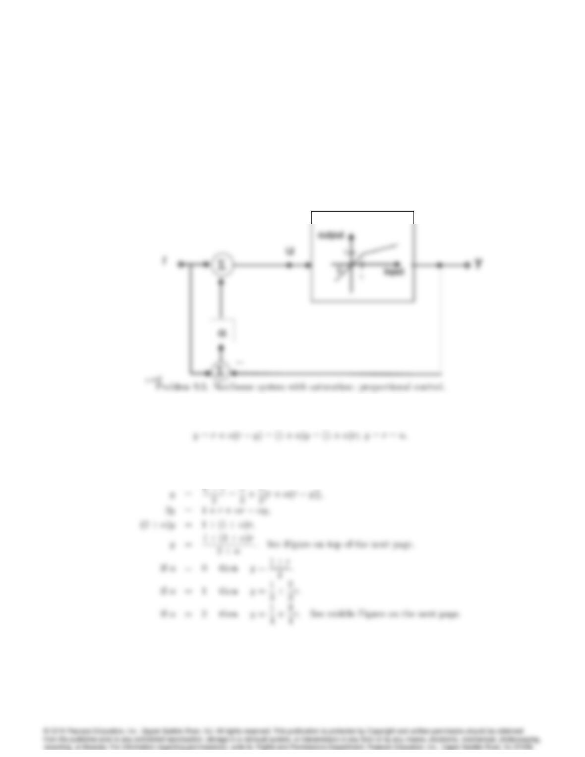
5. Linearizing effect of feedback. We have seen that feedback can reduce the sensitivity of the
input-output transfer function with respect to changes in the plant transfer function , and
reduce the effects of a disturbance acting on the plant. In this problem we explore another
beneficial property of feedback: it can make the input-output response more linear than the
open-loop response of the plant alone. For simplicity let us ignore all the dynamics of the plant,
and assume that the plant is described by the static nonlinearity
y(t) = u u 1
u+1
2u > 1
a) Suppose we use proportional feedback
u(t) = r(t) + (r(t)y(t))
where 0is the feedback gain. Find an expression for y(t)as a function of r(t)for the
closed-loop system (This function is called the nonlinear characteristic of the system.) Sketch
the nonlinear transfer characteristic for = 0 (which is really open-loop), = 1, and = 2.
b) Suppose we use integral control,
u(t) = r(t) + Zt
0
(r()y())d
9008 CHAPTER 9. NONLINEAR SYSTEMS
The closed-loop system is therefore nonlinear and dynamic. Show that if r(t)is a constant, say
r, then lim
t!1y(t) = r. Thus, the integral control makes the steady-state transfer characteristic
of the closed-loop system exactly linear. Can the closed-loop system be described by a transfer
function from rto y?
Solution:
(a)
Fig 10
For u1:
For u > 1:
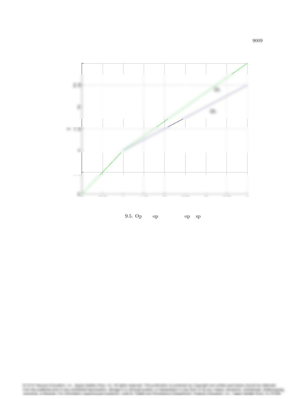
00.5 11.5 22.5 33.5 4
0.5
3
Open-loop vs closed–loop
r
00.5 11.5 22.5 33.5 4
0.5
3
Open-loop vs closed–loop
r
Problem en-lo vs closed-lo re onse.
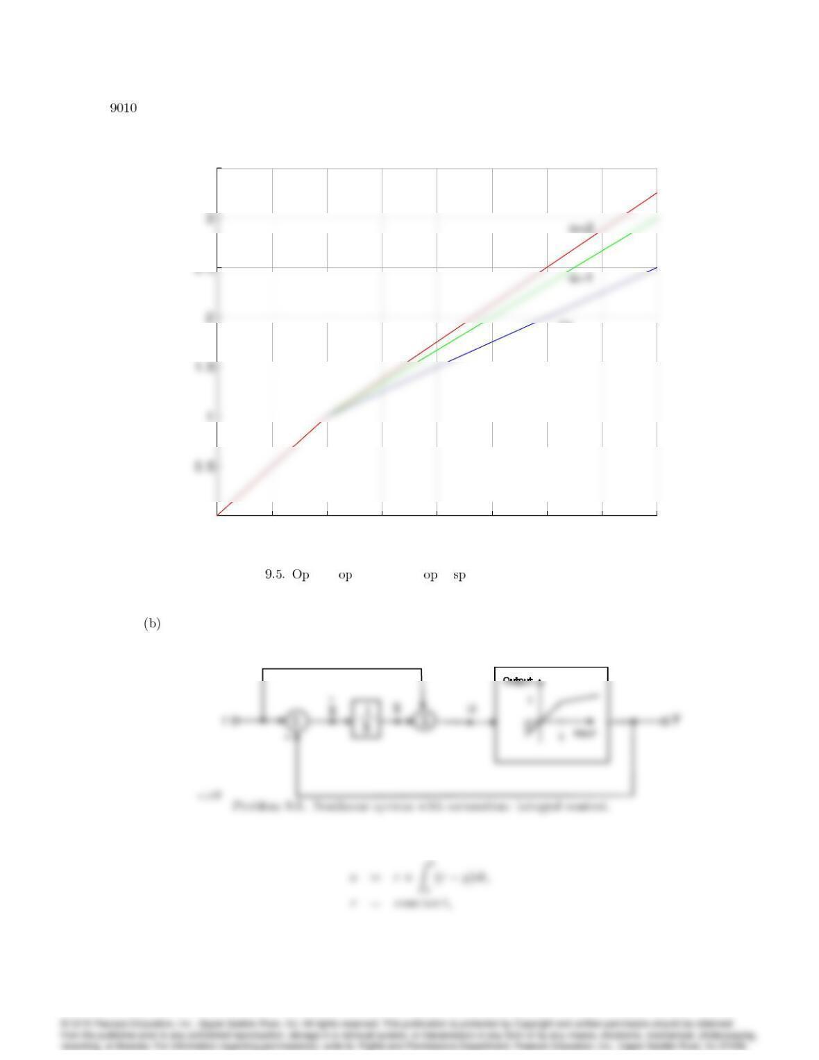
CHAPTER 9. NONLINEAR SYSTEMS
00.5 11.5 22.5 33.5 4
0
3.5
Open-loop vs closed–loop for variousα
r
y
OL
00.5 11.5 22.5 33.5 4
0
3.5
Open-loop vs closed–loop for variousα
r
y
OL
Problem en-lo vs closed-lo re onse for various values of :
Fig 11
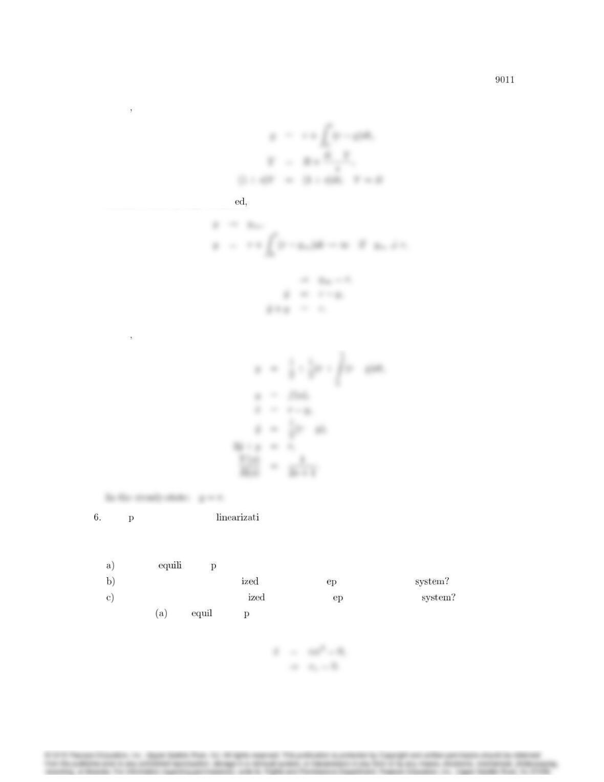
u < 1
Assume stable: ystays bound
u > 1
This roblem shows that on does not always work. Consider the system
_x=x3x(0) 6= 0
Find the brium oint and solve for x(t).
Assume = 1. Is the linear model a valid r resentation of the
Assume =1. Is the linear model a valid r resentation of the
Solution: The ibrium oint is found from:
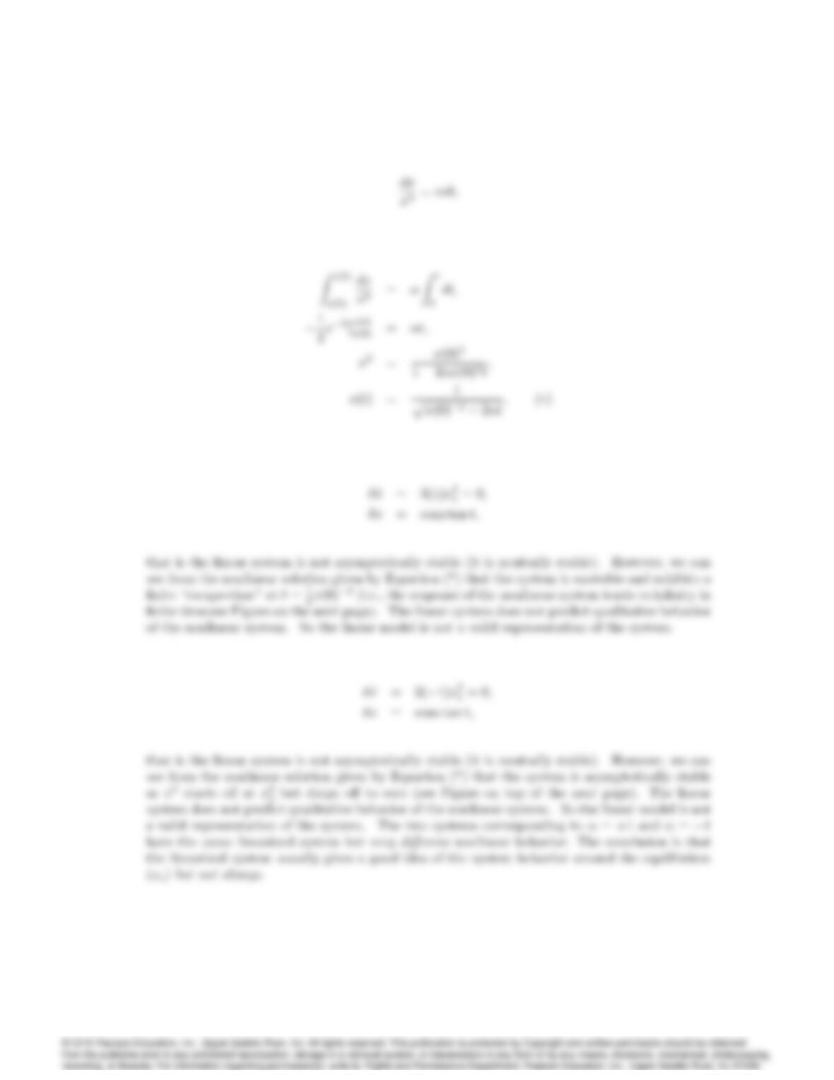
9012 CHAPTER 9. NONLINEAR SYSTEMS
To determine x(t)we re-write the system equation as,
Integrating both sides:
(b) If = 1 the linearized system is,
(c) If =1the linearized system is
020 40 60 80 100
0
1.5
2.5
Time (sec)
020 40 60 80 100
0
1.5
2.5
Time (sec)
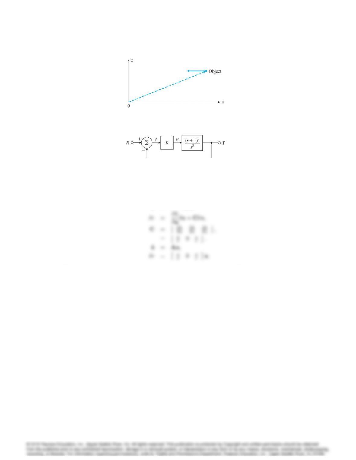
7. Consider the object moving in a straight line with constant velocity shown in Figure 9.60. The
only available measurement is the range to the object. The system equations are
2
4
_x
_v
_z3
5=2
4
010
000
0003
52
4
x
v
z3
5
where
z=cons tan t
_x=cons tan t=v0
r=px2+z2
Derive a linear model for this system.
9014 CHAPTER 9. NONLINEAR SYSTEMS
Figure 9.60: Diagram of moving object for Problem 9.7.
Figure 9.61: Control system for Problem 9.8.
Solution: This system has only an output nonlinearity,
y=r=h(x);
Problems and Solutions for Section 9.3: Equivalent Gain
Analysis Using Root Locus
8. Consider the third-order system shown in Fig. 9.61.
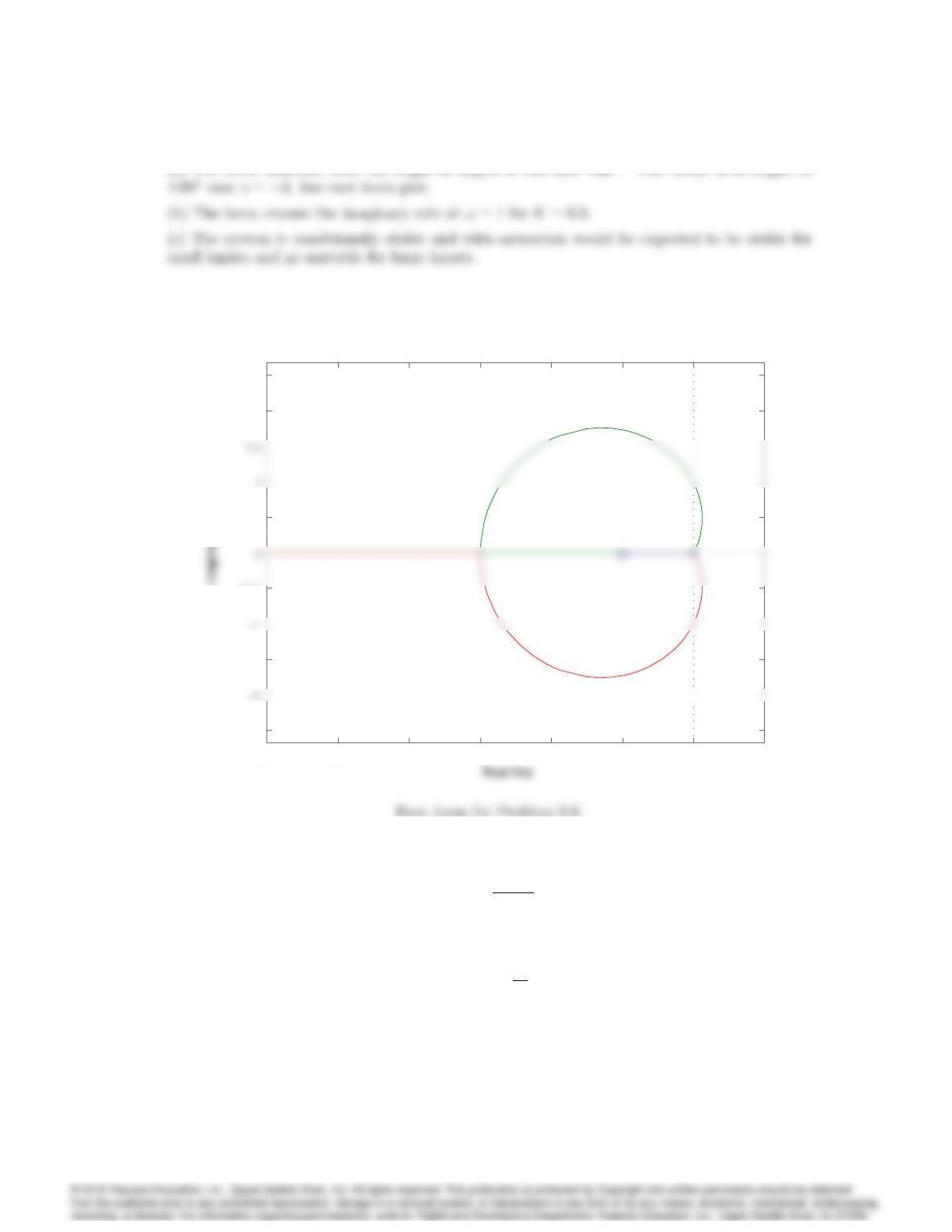
(a) Sketch the root locus for this system with respect to K, showing your calculations for the
asymptote angles, departure angles, and so on.
(b) Using graphical techniques, locate carefully the point at which the locus crosses the imag-
inary axis. What is the value of Kat that point?
(c) Assume that, due to some unknown mechanism, the amplifier output is given by the fol-
lowing saturation non linearity (instead of by a proportional gain K):
u=8
<
:
e; jej 1;
1; e > 1;
1; e < 1:
Qualitatively describe how you would expect the system to respond to a unit step input.
Solution:
9015
-6 -5 -4 -3 -2 -1 0 1
–2.5
–1.5
–0.5
0.5
2
2.5
Root Locus
9. [NEW] Consider the system with the plant transfer function
G(s) = 1
s2+ 1:
We would like to use PID control of the form
Dc(s) = 10 1 + 1
2s+ 2s;
to control this system. It is known that the system’s actuator is a saturation nonlinearity with
a slope of unity and juj 10. Compare the system response for a step input of size 10 with and
9016 CHAPTER 9. NONLINEAR SYSTEMS
without antiwindup circuit. Plot both the step response and the control effort using Simulink.
Qualitatively describe the effect of the antiwindup circuit.
Solution: The Simulink implementation is shown in the ensuing figure.
14:pdf
Simulink diagram for Problem 9.9.
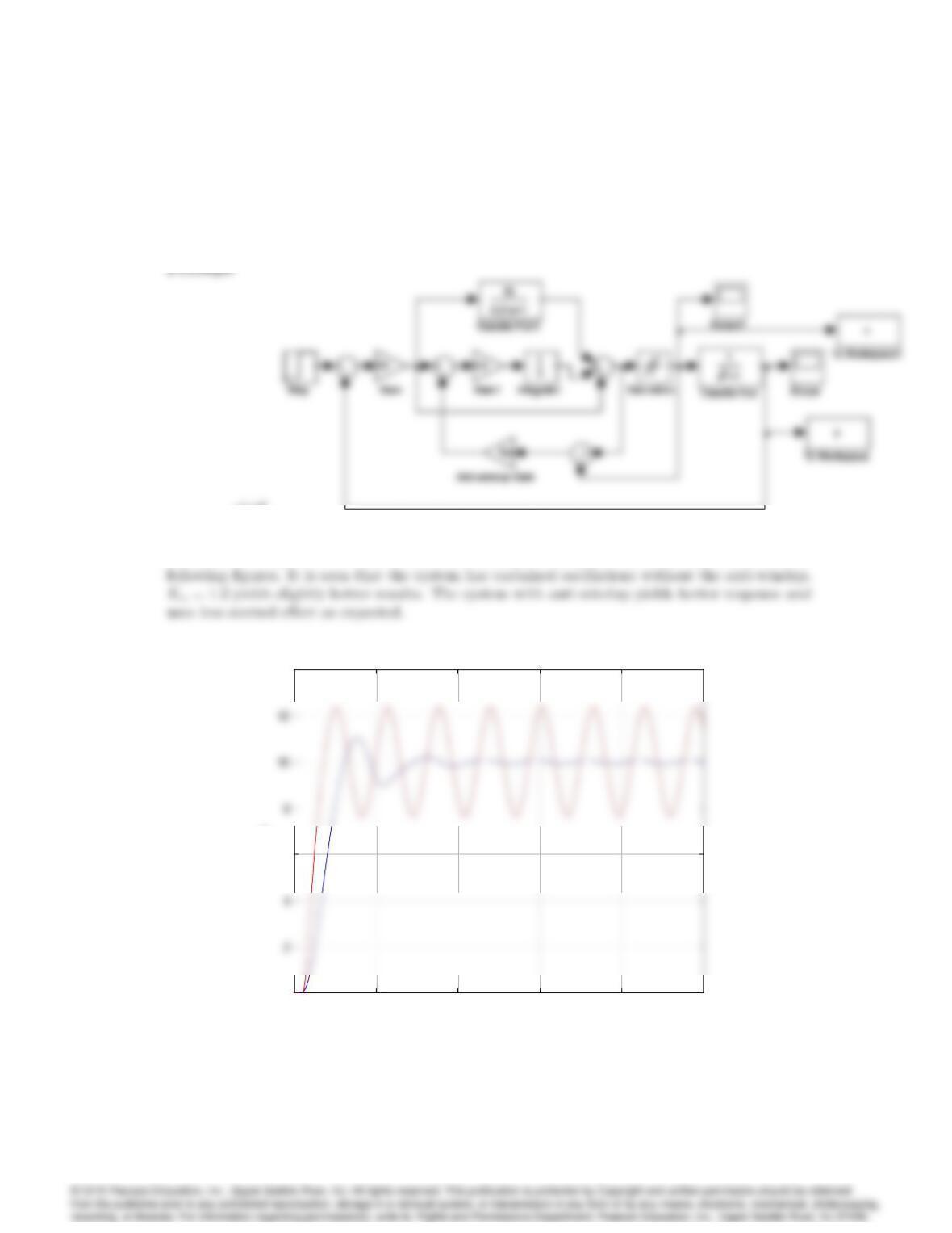
The system’s response with and without anti-windup circuit (Ka= 1; Ka= 0) is shown in the
010 20 30 40 50
0
6
14
Time (sec)
y
010 20 30 40 50
0
6
14
Time (sec)
y
Step responses for Problem 9.9.
9017
010 20 30 40 50
–10
-8
-4
0
6
Time (sec)
u
010 20 30 40 50
–10
-8
-4
0
6
Time (sec)
u
Figure 9.62: Control efforts for Problem 9.9.
(a) Problems and Solutions for Section 9.4: Equivalent Gain
Analysis Using Frequency Response: Describing Func–
tions
10. Compute the describing function for the relay with deadzone nonlinearity shown in Figure 9.6
(c).
Solution:
Y1=1
Z2
0
y(t) sin(!t)d(!t)
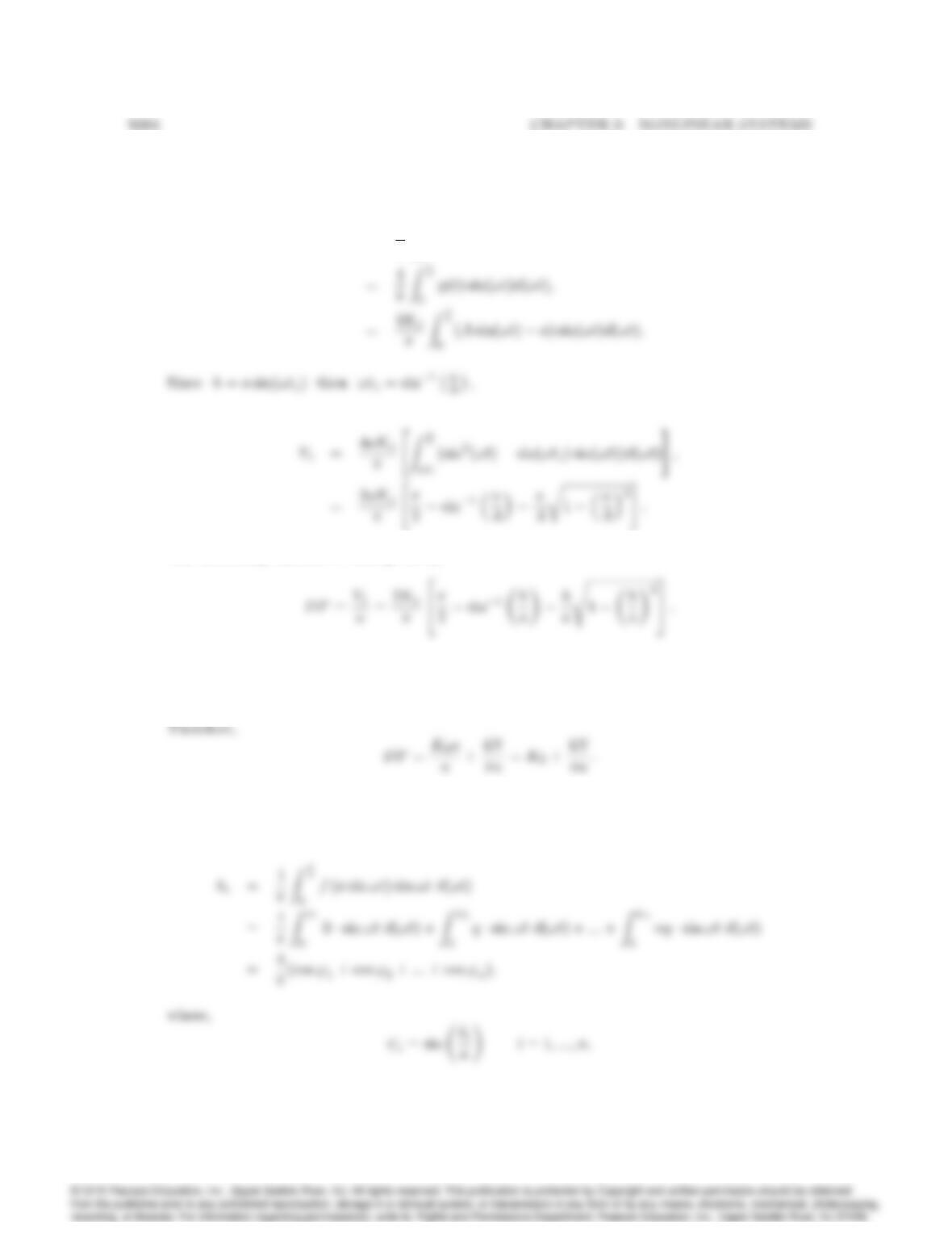
11. Compute the describing function for gain with dead zone nonlinearity shown in Figure 9.6 (d).
Solution: This is an odd nonlinearity so that all the cosine terms are zeros and the DF is real:
Y1=1
Z2
0
y(t) sin(!t)d(!t);
The describing function is then given by,
12. Compute the describing function for the preloaded spring or Coulomb plus viscous friction
nonlinearity shown in Figure 9.6 (e).
Solution: This is a combination of a gain, K0, plus a relay nonlinearity (see Example 9.11).
13. Consider the quantizer function shown in Figure 9.63 that resembles a staircase. Find the
describing function for this nonlinearity and write a Matlab .m function to generate it.
Solution. The abscissa breakpoints are denoted by i. From Eq. 9.23,
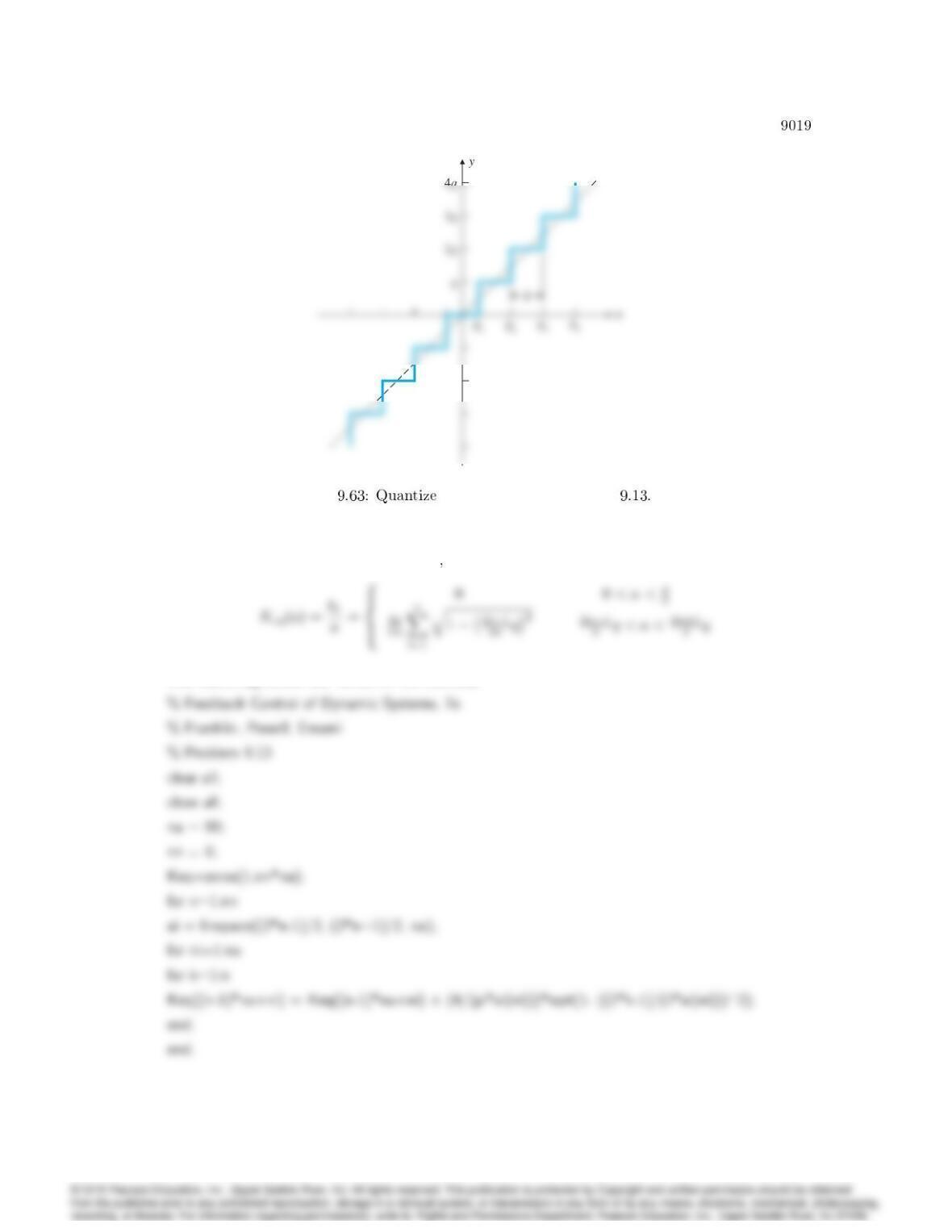
Figure r nonlinearity for Problem
The describing function is then given by
The following shows the Matlab .m function: