Operating Systems Chapter 9 Homework First Investigate The Equilibrium Points Next Investigate

9040 CHAPTER 9. NONLINEAR SYSTEMS

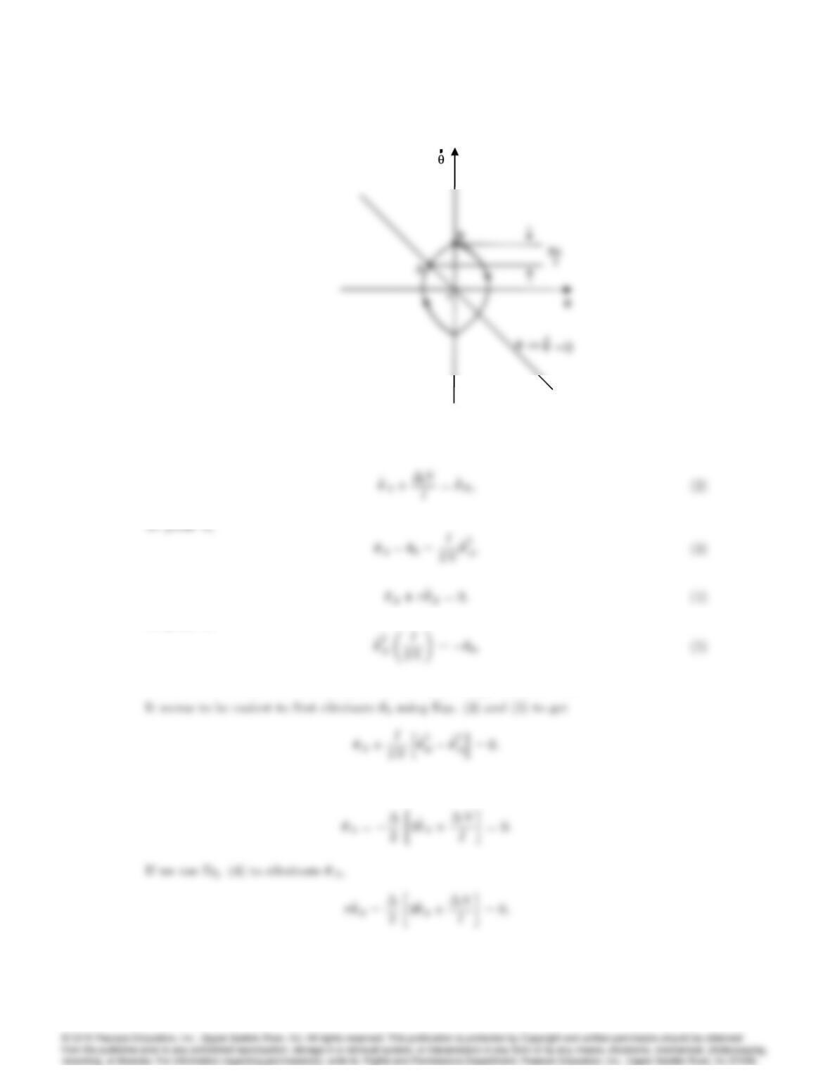
Fig 6

38:pdf

Phase-plane trajectory of limit cycle for Problem 9.22.

From the geometry of the limit cycle (see above Figure),

At point B,

We need to solve the above four equations for 0(for max =0,0= 0).

If we eliminate _

Busing Eq. (2), then,

9041

Solve for _

A,

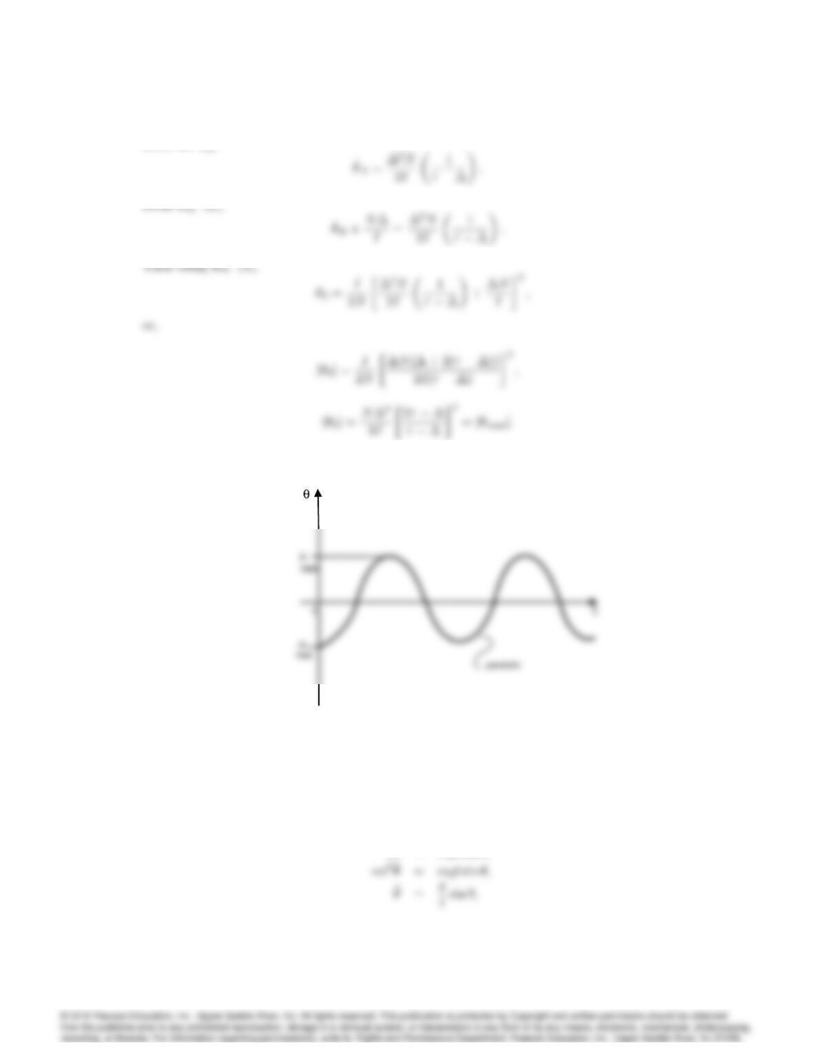
Time history shown in the Figure below and shows a “nonlinear oscillator.”

Fig 7

39:pdf

Nonlinear oscillator for Problem 9.22.

23. Consider the point mass pendulum with zero friction as shown in Figure 9.67. Using the method

of isoclines as a guide, sketch the phase-plane portrait of the motion. Pay particular attention

to the vicinity of =. Indicate a trajectory corresponding to spinning of the bob around and

around rather than oscillating back and forth.

(a) Solution: The equations are:

I•

=mgl sin ;

9042 CHAPTER 9. NONLINEAR SYSTEMS

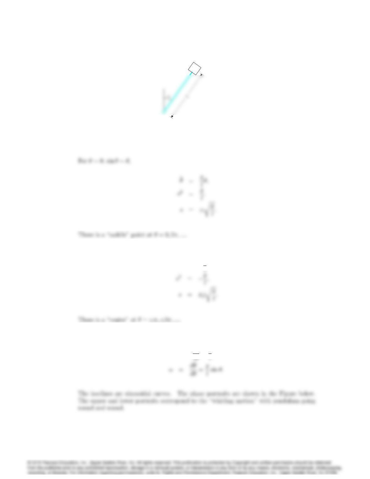
M

Figure 9.67: Pendulum for Problem 9.23.

For ,sin  ;

•

=g

Using isoclines:

•

=_

d_



9043

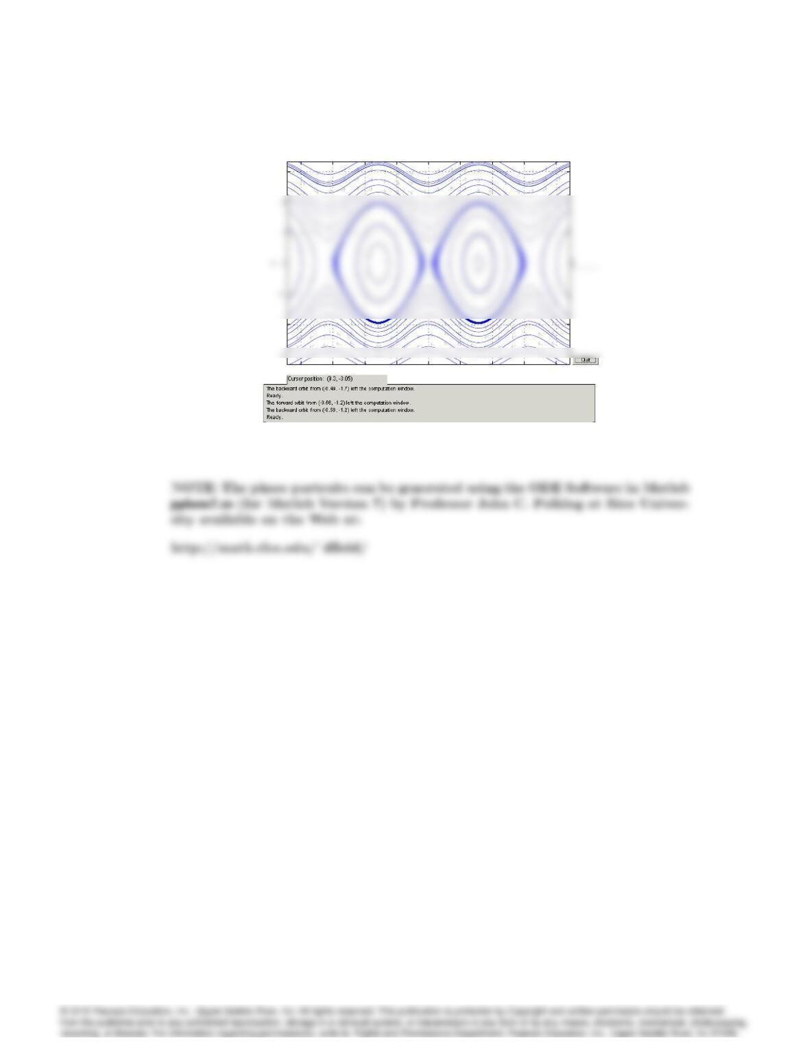
x ‘ = y

y ‘ = sin(x)

-8 -6 -4 -2 0 2 4 6 8

-2

3

x

Phase portraits for Problem 9.23.

24. Draw the phase trajectory for a system

•x= 106m/ sec2

between _x(0) = 0,x(0) = 0 and x(t) = 1mm. Find the transition time, tf, by graphical means

from the parabolic curve by comparing your solution with several different interval sizes and the

exact solution.

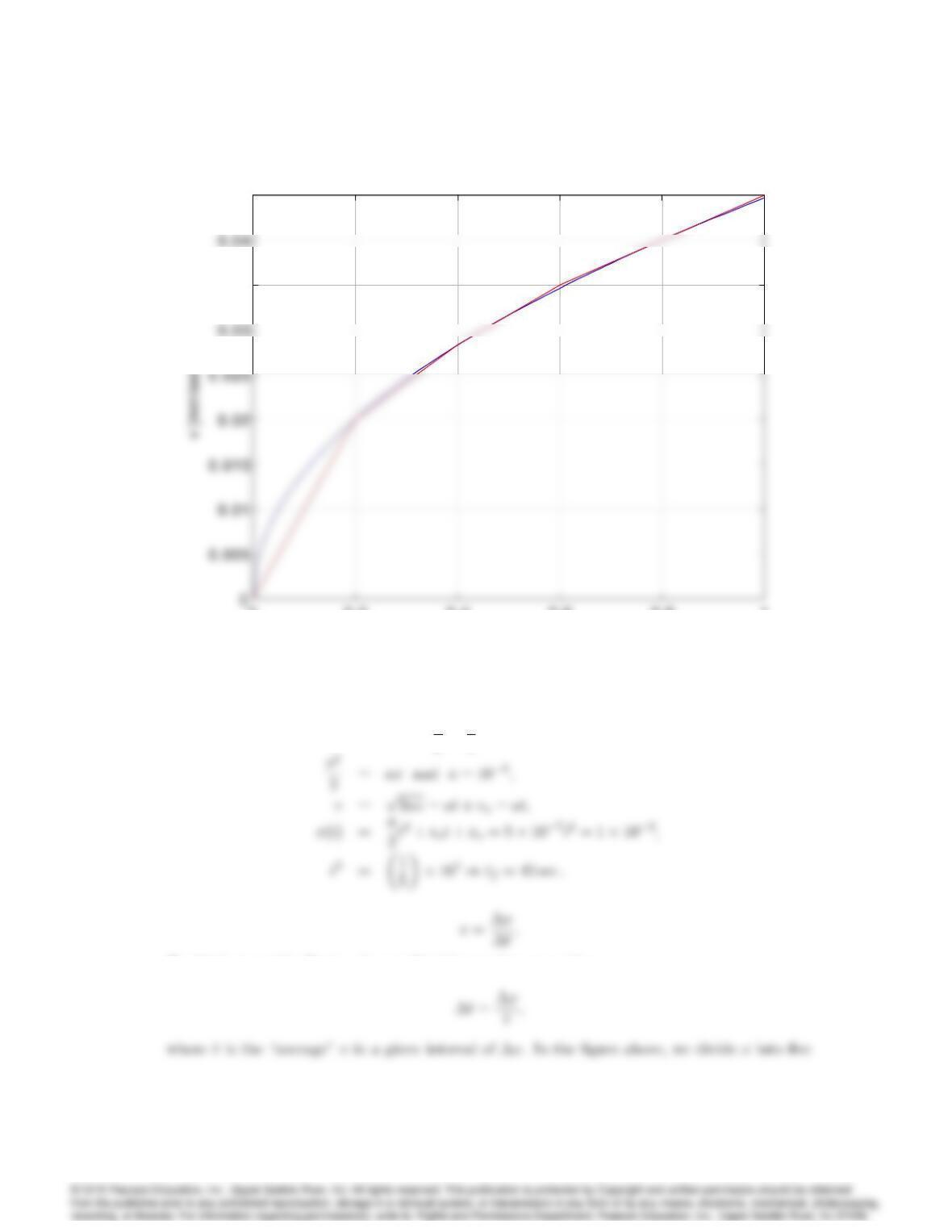
Solution: The phase portrait is shown in the figure below.

9044 CHAPTER 9. NONLINEAR SYSTEMS

00.2 0.4 0.6 0.8 1

0.035

0.045

x [mm]

Phase portrait

00.2 0.4 0.6 0.8 1

0.035

0.045

x [mm]

Phase portrait

Phase portrait for Problem 9.24.

•x=a; _v

_x=a

v;

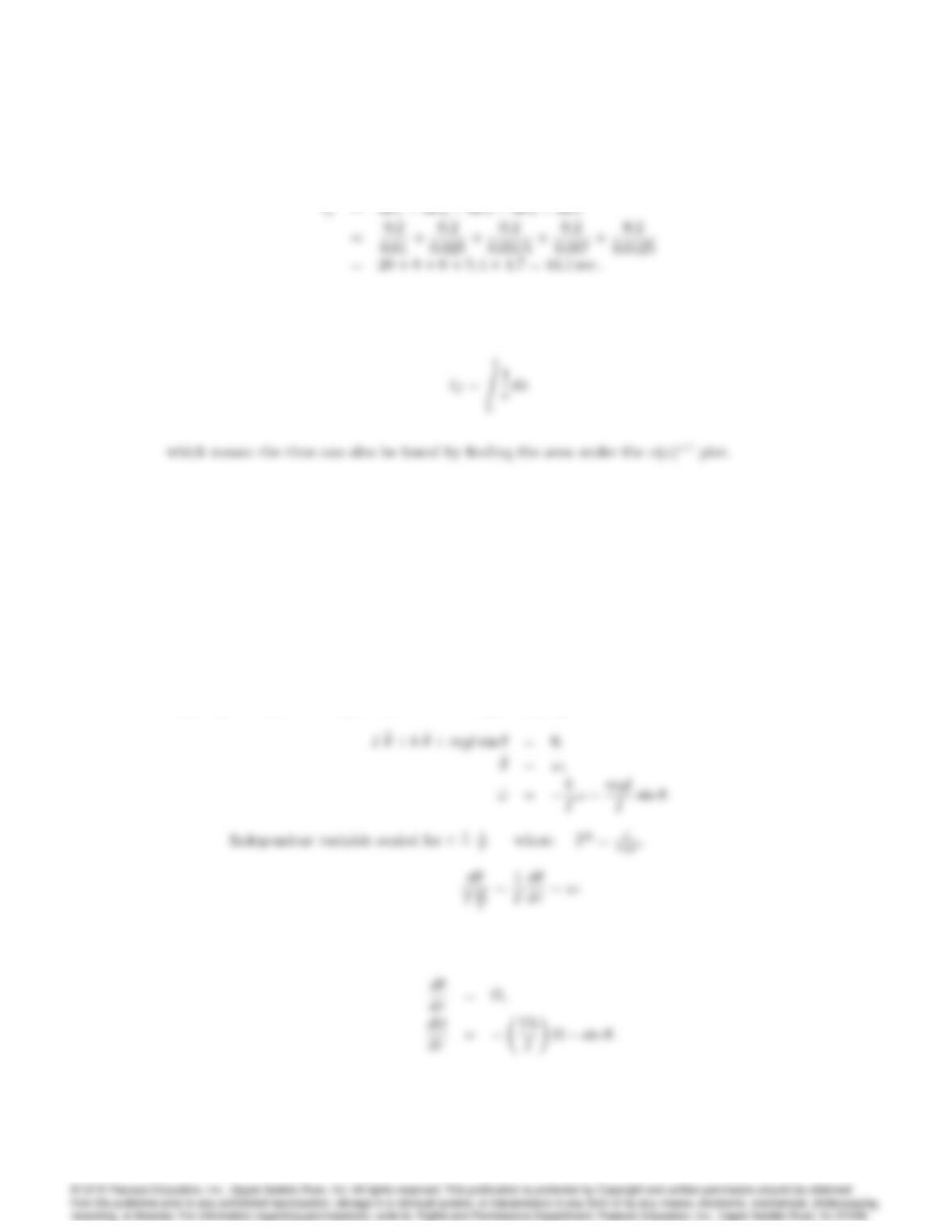
To obtain tgraphically, i.e., by graphical integration, we write,

9045

intervals and find (going from left to the right),

tf= t1+ t2+ t3+ t4+ t5

which compares well with the exact answer of t= 45 sec. Better approximation can be found

by finer division of x. Alternatively we can compute the time from,

25. Consider the system with equations of motion,

•

+_

+ sin = 0

a) What physical system does this correspond to?

b) Draw the phase portraits for this system.

c) Show a specific trajectory for 0= 0:5rad _

= 0.

Solution:

(a) Physical system is a pendulum with a hinge damping.

Let us define ,T !.

9046 CHAPTER 9. NONLINEAR SYSTEMS

Fig 5

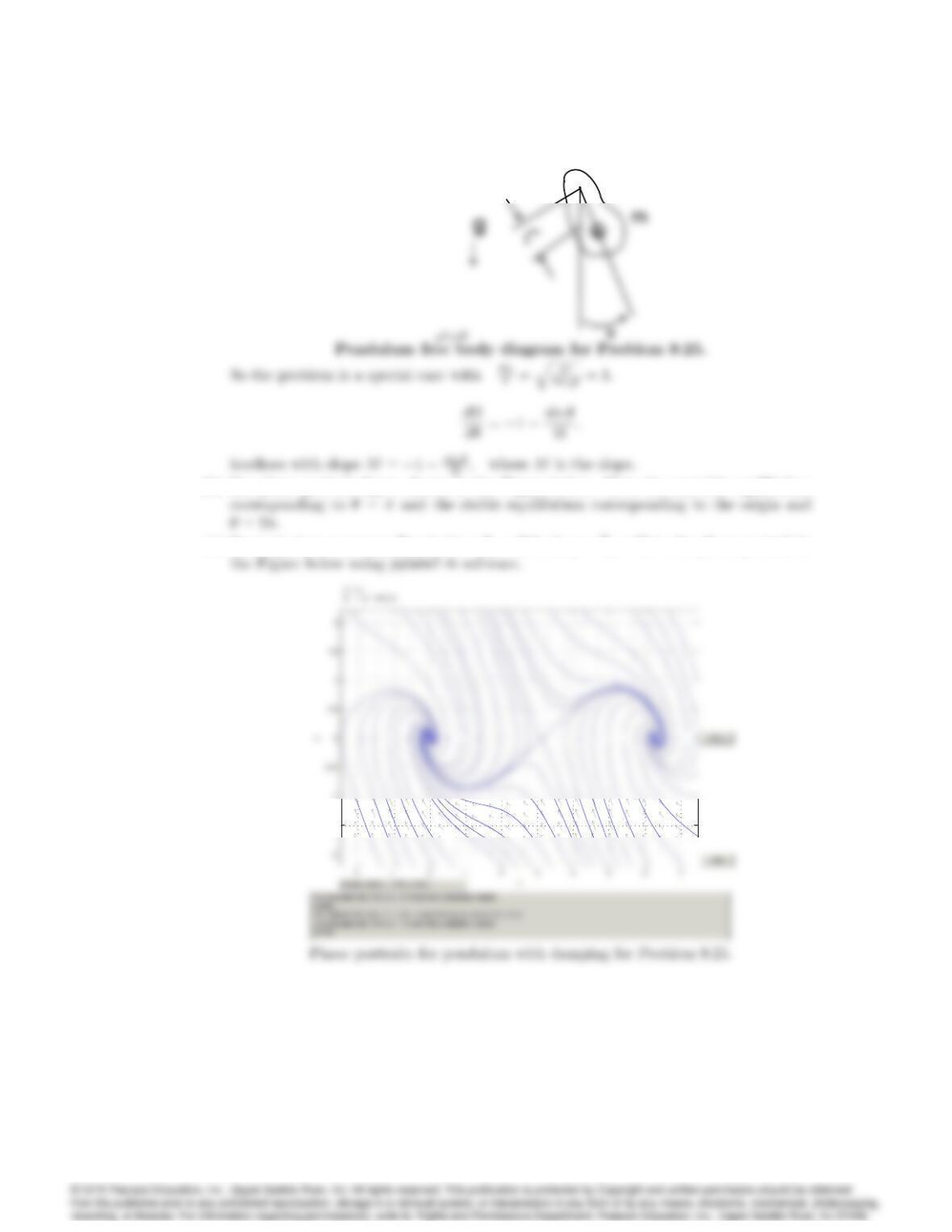
(b) See phase portrait figure shown in the Figure below. Note the unstable equilibrium

(c) See trajectory corresponding to (x=0= 0:5rad; y =_

0= 0) in the phase portrait in

– 1 .5

-1

26. Consider the nonlinear upright pendulum with a motor at its base as an actuator. Design a

feedback controller to stabilize this system.

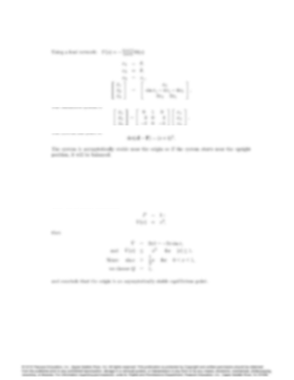
Solution: •

= sin +u:

9047

27. Consider the system

_x=sin x

Prove that the origin is an asymptotically stable equilibrium point.

Solution:We wish to show that _

V(x) xTQx.

Select the Lyapunov function for

28. A first-order nonlinear system is described by the equation _x=f(x), where f(x)is a continuous

and differentiable nonlinear function that satisfies the following:

f(0) = 0;

f(x)>0 for x > 0;

f(x)<0 for x < 0:

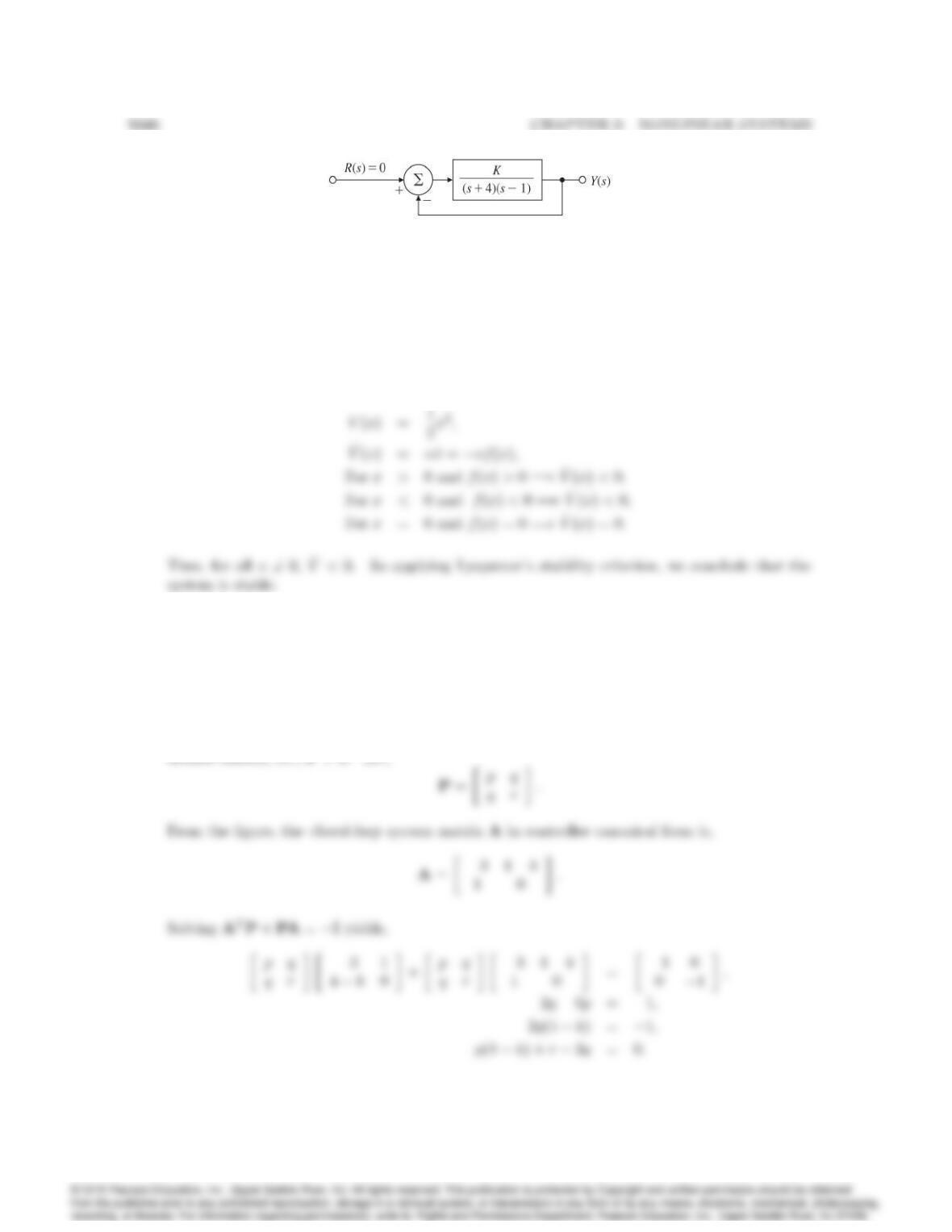
Figure 9.68: Control system for Problem 29

Use the Lyapunov function V(x) = x2=2to show that the system is stable near the origin

(x= 0).

Solution:

_x=f(x);

29. Use the Lyapunov equation

ATP+PA =Q=I

to find the range of Kfor which the system in Fig. 9.68 will be stable. Compare your answer

with the stable values for Kobtained using Routh’s stability criterion.

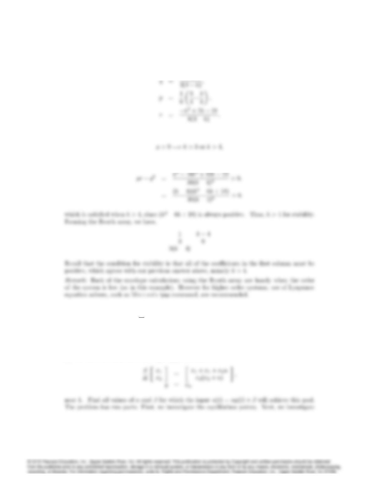
Solution:

Our approach is to set up the continuous Lyapunov equation and check that Pis a positive

9049

Hence,

The two conditions for P>0are p > 0and pr q2>0, or,

and,

30. Consider the system

d

dt x1

x2=x1+x2u

x2(x2+u); y =x1:

Find all values of and for which the input u(t) = y(t)+will achieve the goal of maintaining

the output y(t)near 1.

Solution:

(a) It is desired to maintain the output y(t)of the system,

9050 CHAPTER 9. NONLINEAR SYSTEMS

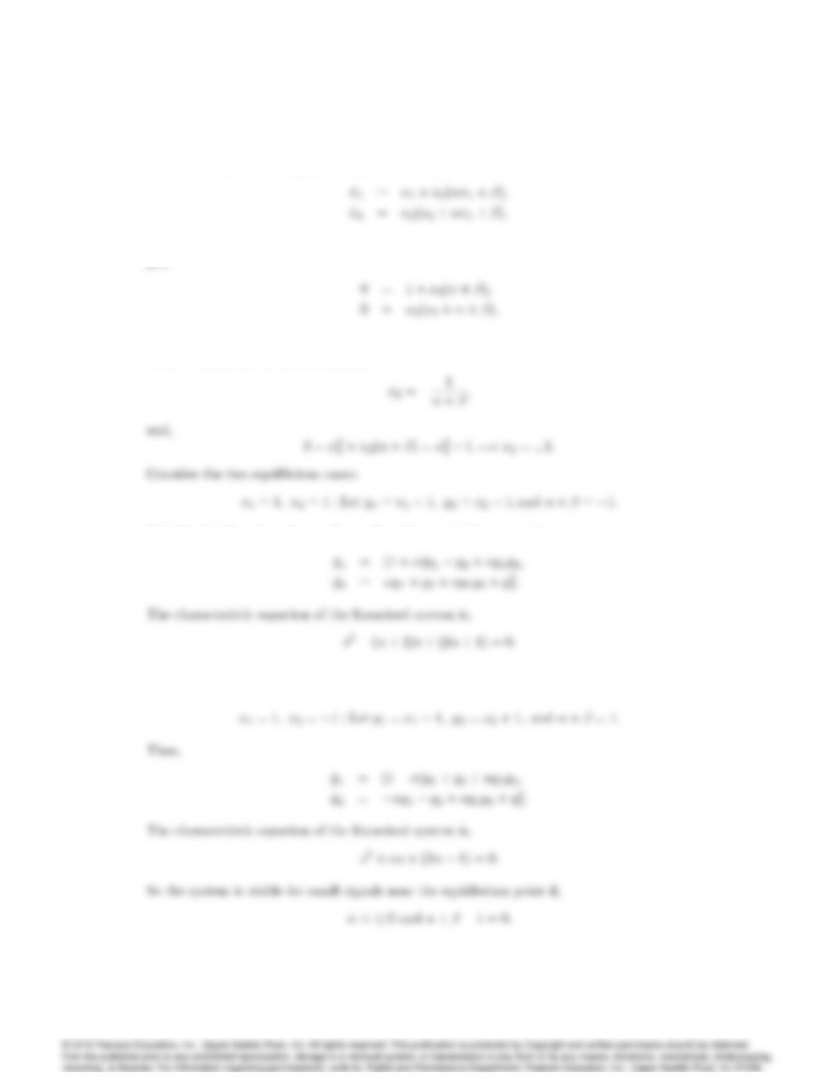
the stability of the system by linearizing the nonlinear state equations near these equilibria.

The nonlinear, closed-loop system equations are,

To find the equilibrium points for the desired output of y= 1, we set x1= 1,_x1= _x2= 0, to

get,

which can be solved for the equilibrium values of x2and the necessary relationship between 

and . Simultaneous solution yields,

Substituting these into the nonlinear closed-loop equations, we get,

There are no values of which produce stable roots. So we conclude x1= 1 and x2= 1 is an

unstable equilibrium point.

31. Consider the nonlinear autonomous system

d

dt 2

4

x1

x2

x33

5=2

4

x2(x3x1)

x2

11

x1x33

5:

a) Find the equilibrium point(s).

b) Find the linearized system about each equilibrium point.

c) For each case in part (b), what does Lyapunov theory tell us about the stability of the

nonlinear system near the equilibrium point?

Solution:

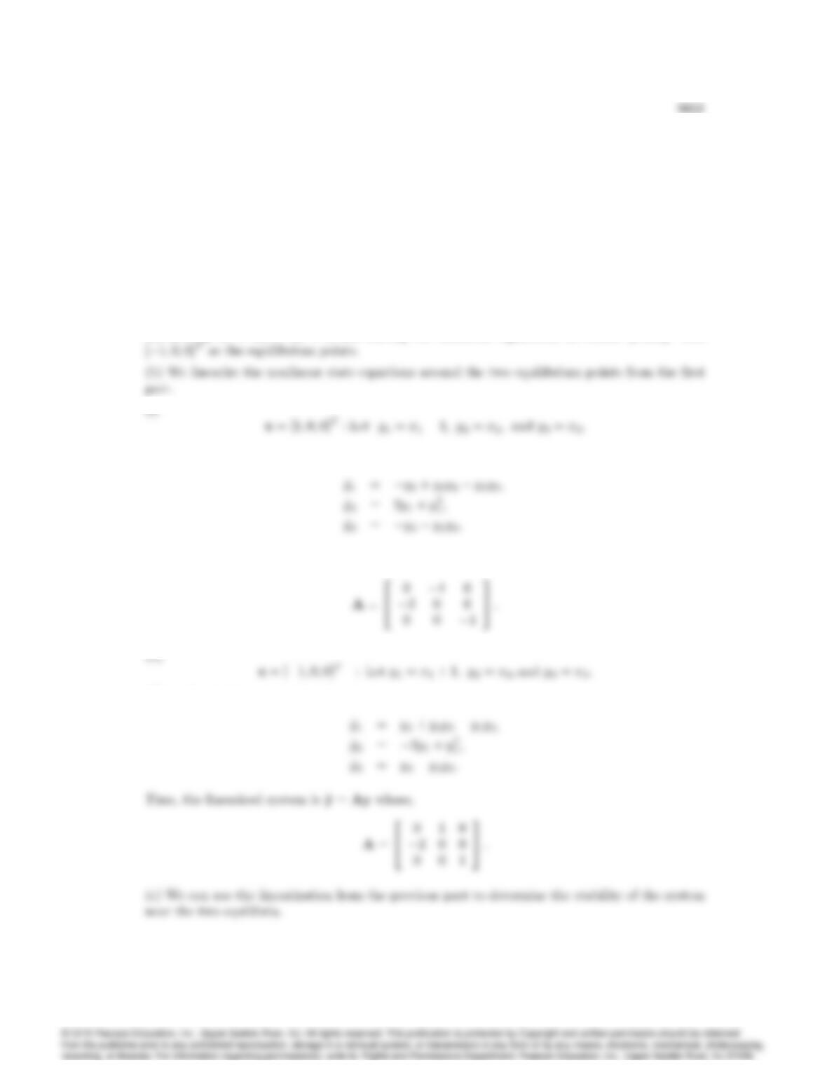
(a) Setting _x1= _x2= _x3= 0 and solving the nonlinear equations, we obtain [1;0;0]Tand

Then the nonlinear equations become,

Thus, the linearized system is _y =Ay where,

Then the nonlinear equations become,

(i) The characteristic equation is (s2+2)(s+1) = 0. The linear system is neutrally (marginally)

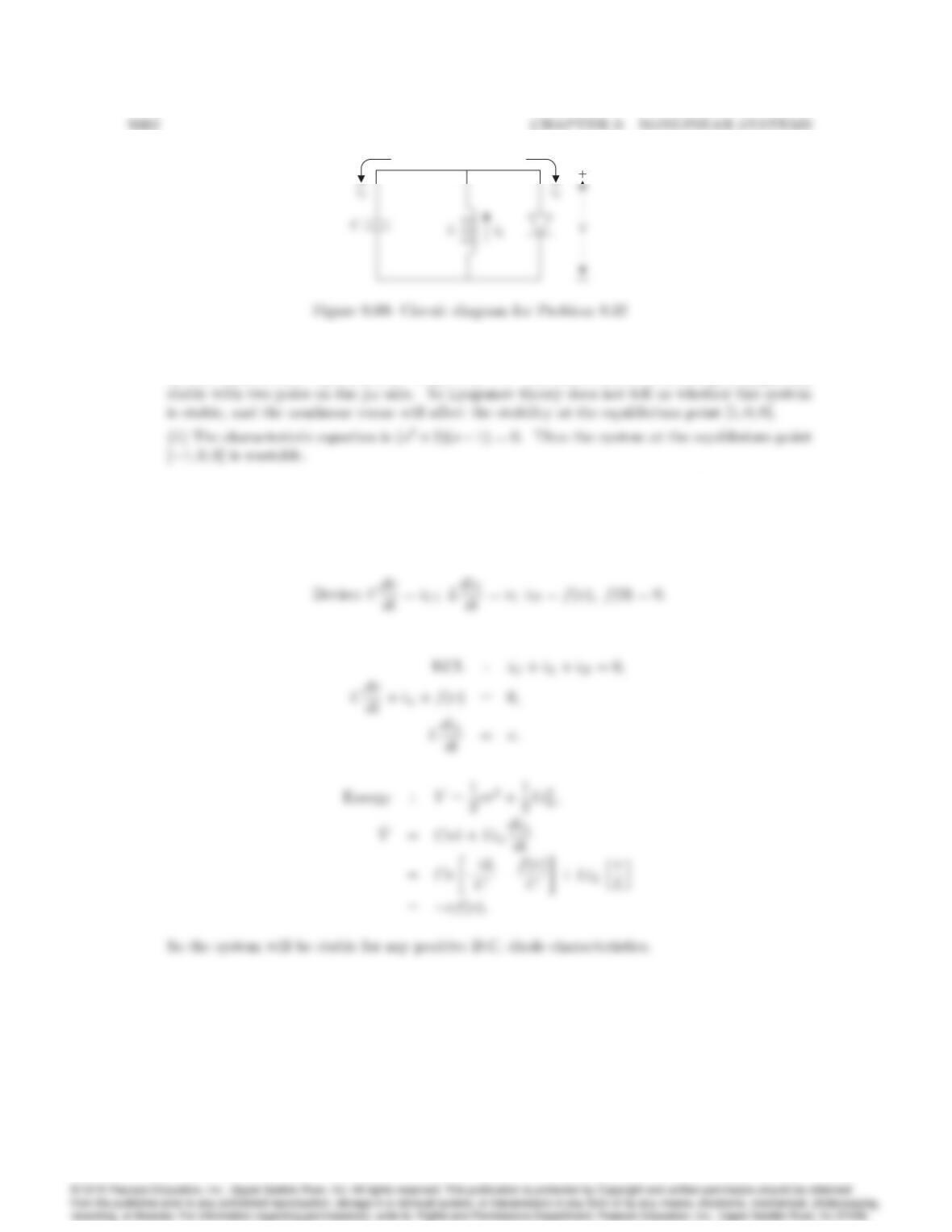
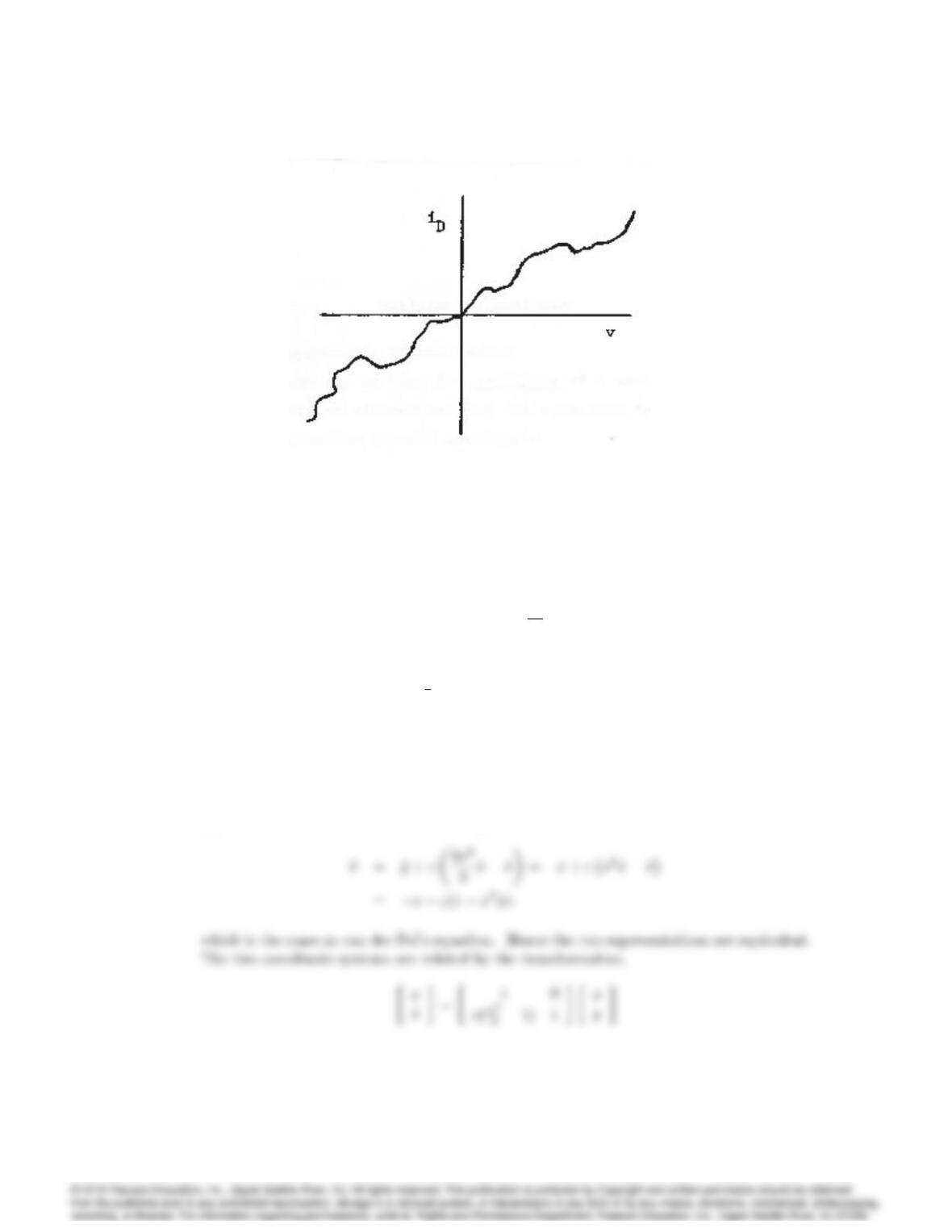
32. Consider the circuit shown in Figure 9.69. For what diode characteristics will this system be

stable?

Solution:

The system equations are:

33. Van der Pol’s equation: Consider the system described by the nonlinear equation

•x+“(1 x2) _x+x= 0

with the constant ” > 0.

9053

Figure 9.70: Diode characteristics.

(a) Show that the equations can be put in the form [Liénard or (x; y) plane]:

_x=y+“x3

3x

_y=x.

(b) Use the Lyapunov function V=1

2(x2+ _x2)and sketch the region of stability as predicted

by this Vin the Liénard plane.

(c) Plot the trajectories of part (b) and show the initial conditions that tend to the origin. Sim-

ulate the system in Simulink R

using various initial conditions on x(0) and _x(0). Consider

two cases with “= 0:5, and “= 1:0.

Solution:

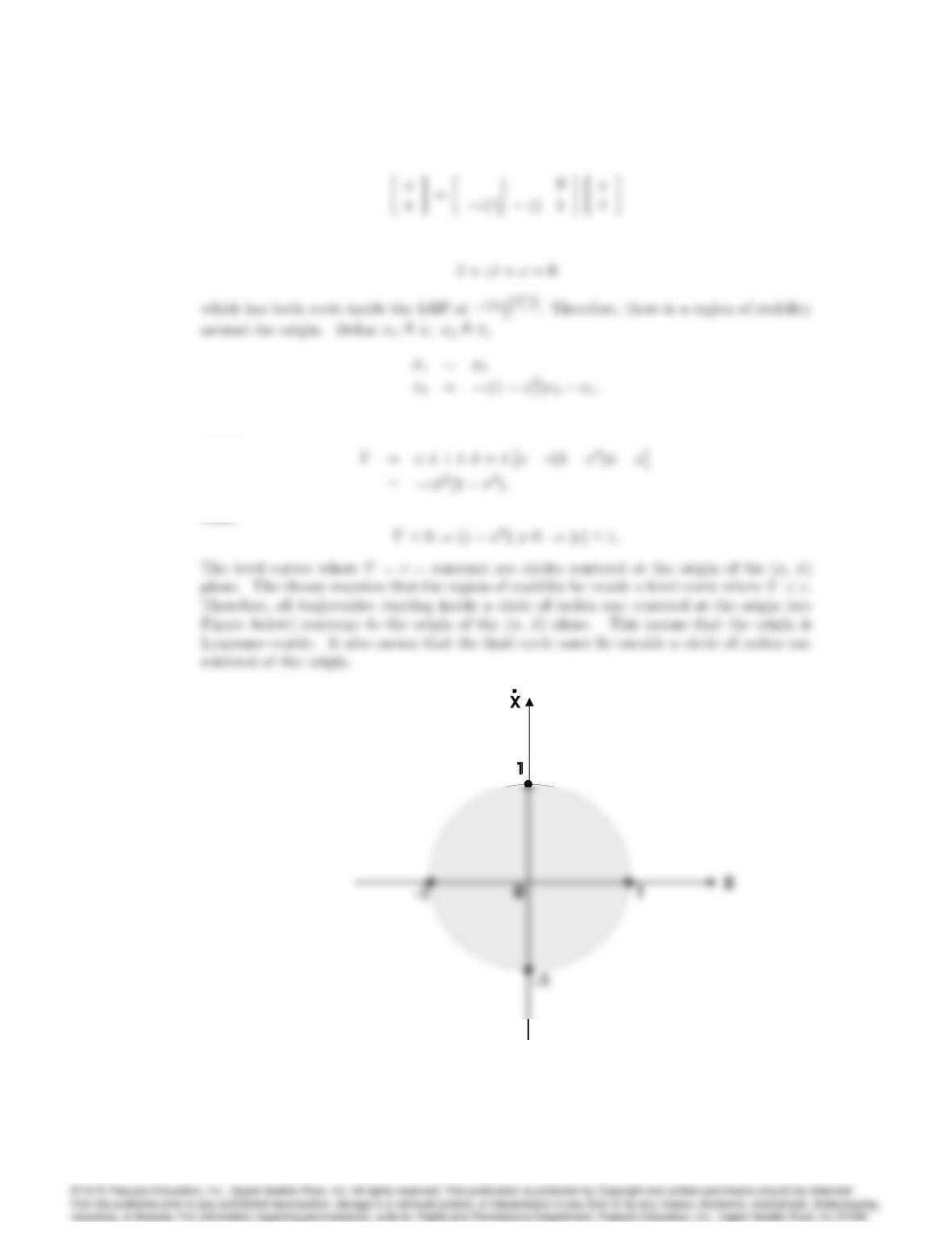
(a) If we differentiate the first Liénard equation, we obtain

or,

9054 CHAPTER 9. NONLINEAR SYSTEMS

(b) If we linearize the system, we obtain

Then,

Fig 18

48:pdf

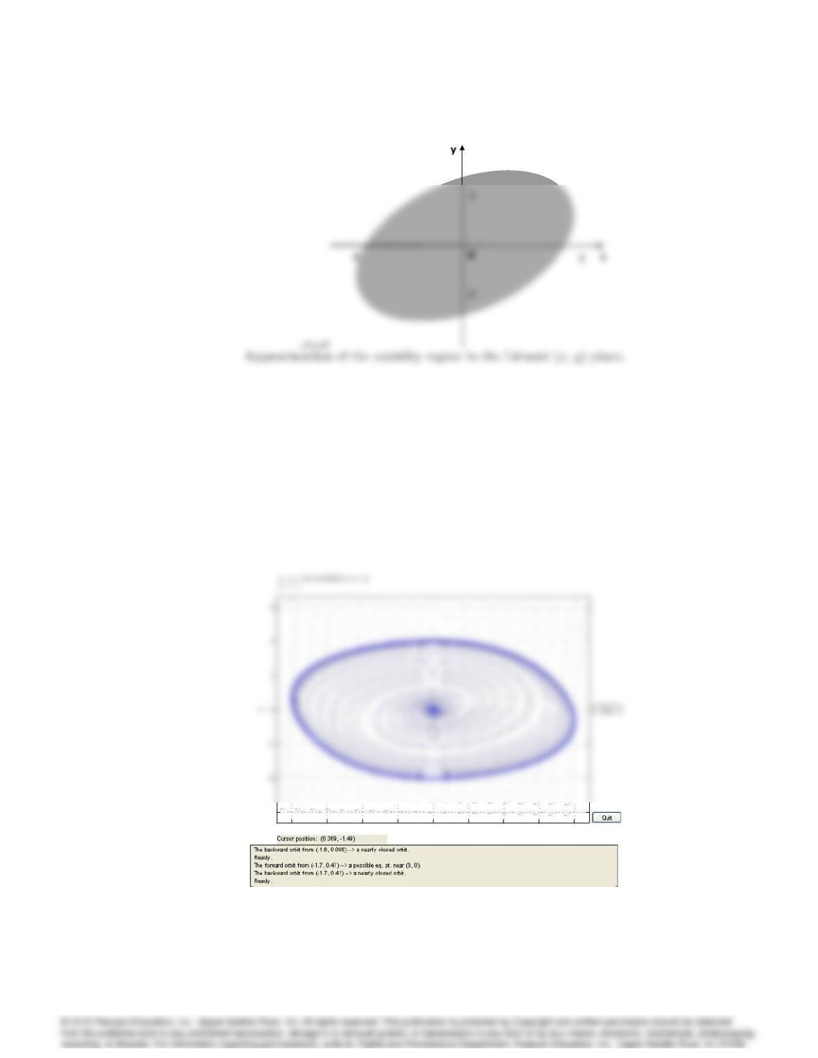
Stability region in the (x,_x) plane.

9055

-2 –1.5 -1 –0.5 00.5 11.5 2

–1.5

1

1.5

x

Stability reg ion

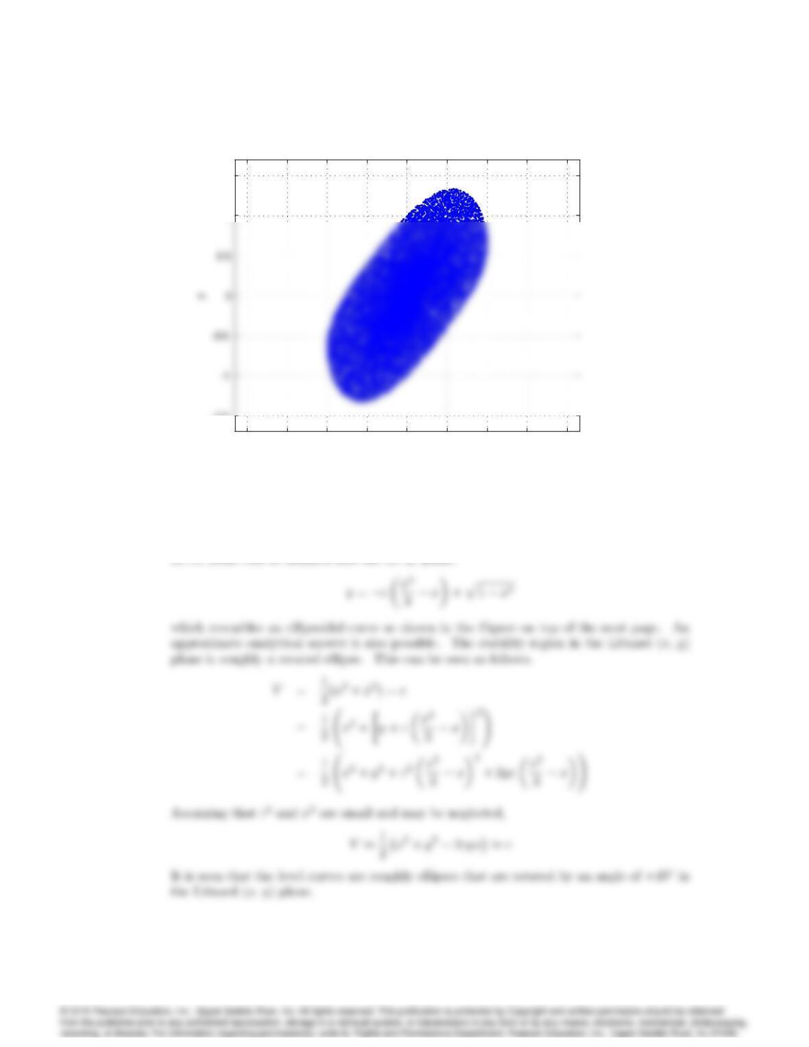
Figure 9.71: Stability region in the Liénard (x,y) plane.

The stability region may be mapped into the Liénard plane. The circular boundary in the

(x,_x) plane can be mapped into the (x,y) plane:

9056 CHAPTER 9. NONLINEAR SYSTEMS

Fig 19

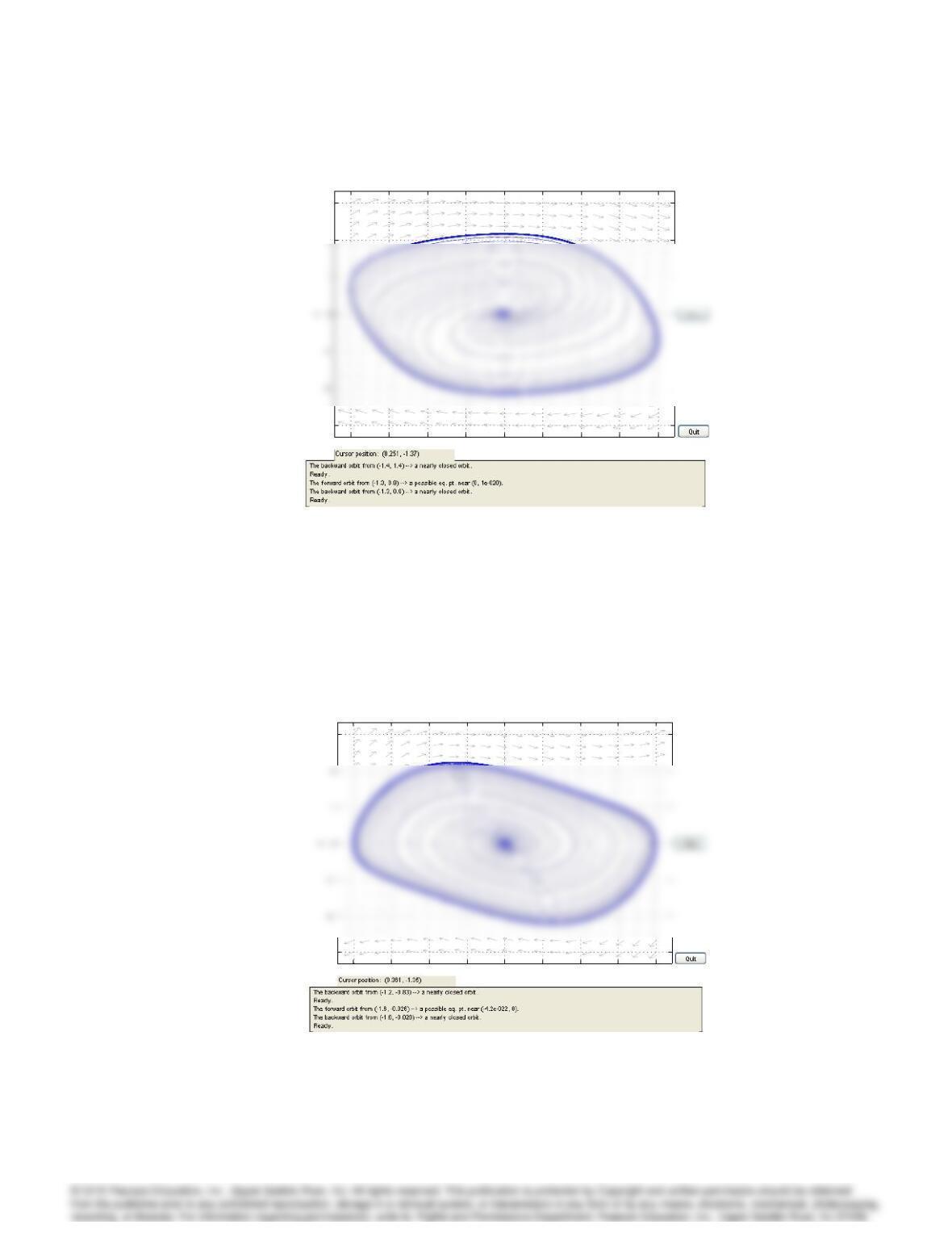
(c) Using pplane7.m software we see that the limit cycle is nearly circular with radius 2:

-2 – 1 .5 -1 – 0 .5 00 .5 11 .5 2

-3

x

Phase portraits for van der Pol equation in Liénard (x,y) form for “= 0:5:

9057

x ‘ = y + (0.33333 x x x – x)

y ‘ = – x

-2 -1.5 -1 -0.5 00.5 11.5 2

-3

2

3

x

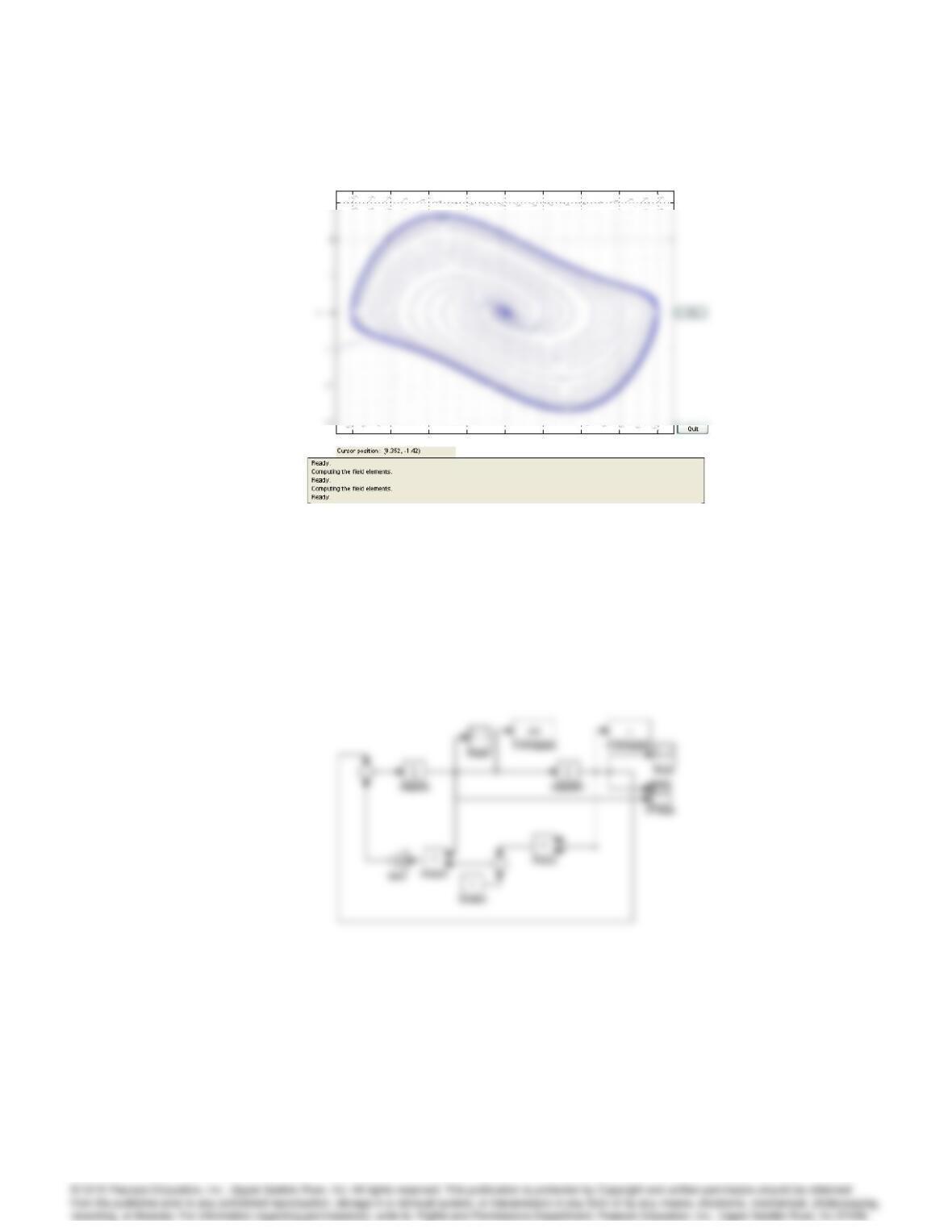
Phase portraits for van der Pol equation in the Liénard (x,y) plane for “= 1:0.

x ‘ = y

y ‘ = – x – 0.5 (1 – x x) y

-2 –1.5 -1 –0.5 00.5 11.5 2

-3

3

x

Phase portraits for van der Pol equation in the (x,_x) plane for “= 0:5.

9058 CHAPTER 9. NONLINEAR SYSTEMS

x ‘ = y

y ‘ = – x – (1 – x x) y

-2 -1.5 -1 -0.5 00.5 11.5 2

-3

3

x

Phase portraits for van der Pol equation in the (x,_x) plane for “= 1:0.

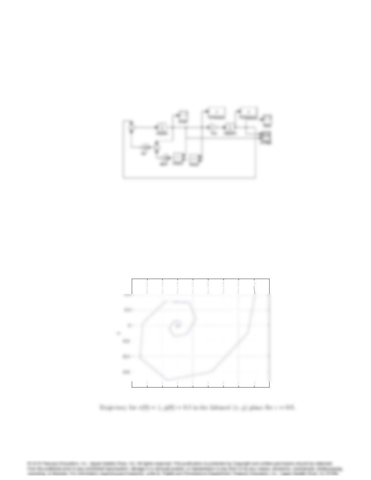
The Simulink simulations are shown in the attached figures.

Simulink simulation diagram for van der Pol’s equation for (x,_x) plane.

9059

Simulink simulation of van der Pol’s equation in the Liénard (x,y) plane.

Sample trajectories are shown in the attached figures.

–0.6 –0.4 –0.2 00.2 0.4 0.6 0.8 11.2

–0.8

0.6

x