Operating Systems Chapter 9 Homework Derive the describing function for the ideal contactor controller

9020 CHAPTER 9. NONLINEAR SYSTEMS

end;

0.6

1.4

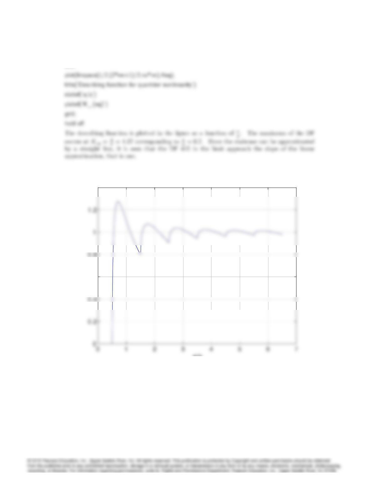
Describing function for quantizer nonlinearity

a/q

Keq

0.6

1.4

Describing function for quantizer nonlinearity

a/q

Keq

Describing function for quantizer nonlinearity

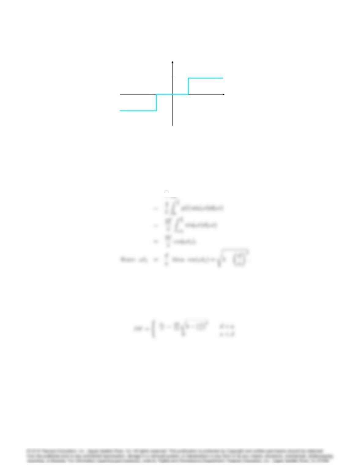
14. Derive the describing function for the ideal contactor controller shown in Figure 9.64. Is it

frequency dependent? Would it be frequency dependent if it had a time delay or hysteresis?

Graphically, sketch the time histories of the output for several amplitudes of the input and

determine the describing function values for those inputs.

9021

O u t p u t

I n p u t

d

T

Figure 9.64: Contactor for Problem 9.14

Solution:

Y1=1

Z2

y(t) sin(!t)d(!t)

The describing function is then given by,

and is not frequency dependent. See Figure on top of the next page. Frequency dependence

will be introduced with a delay.

9022 CHAPTER 9. NONLINEAR SYSTEMS

0 1 2 3 4 5

0

1

4

7

a

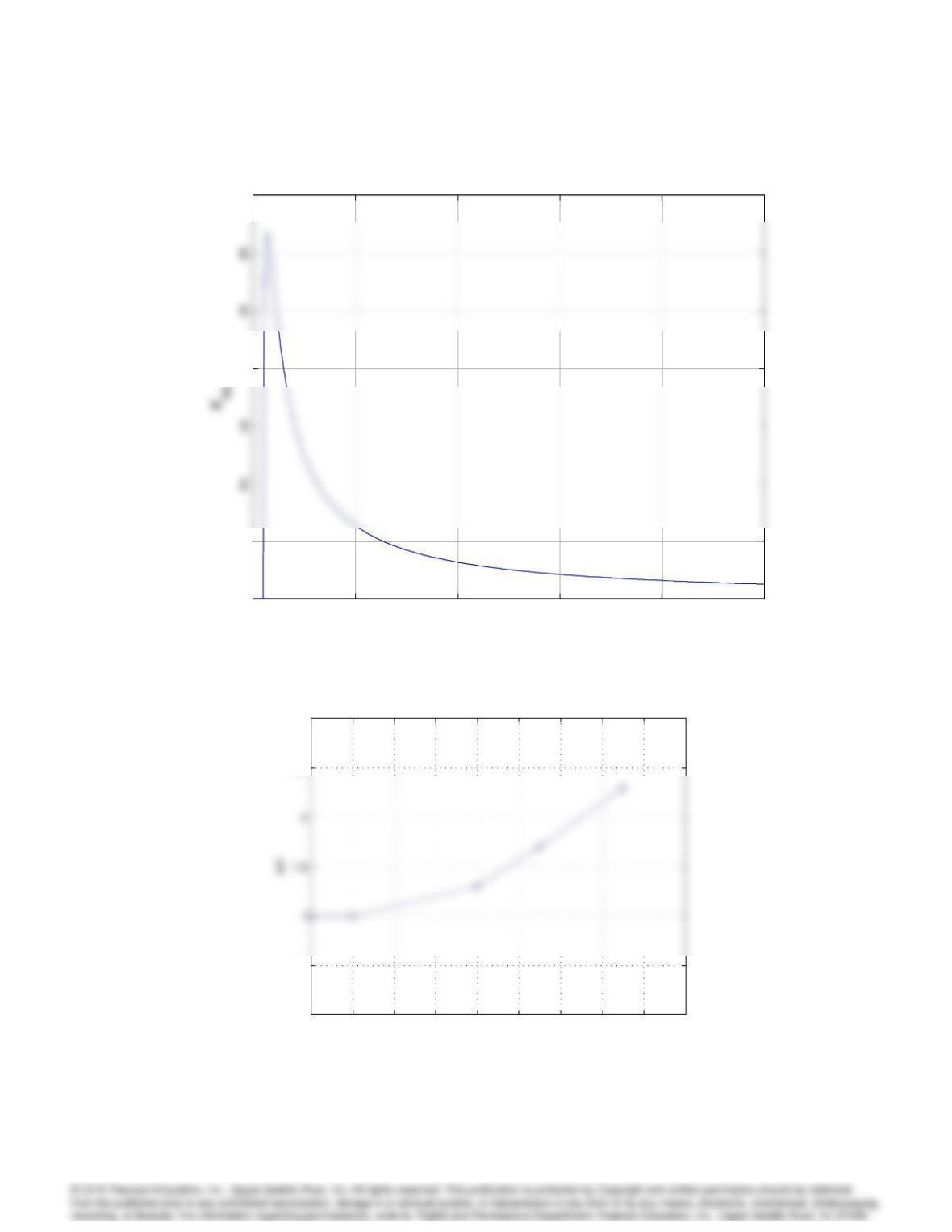
Describing function: DF

0 1 2 3 4 5

0

1

4

7

a

Describing function: DF

Problem 9.14. DF for d= 0:1,T= 1:0.

010 20 30 40 50 60 70 80 90

0

0.5

2.5

3

ω t0

9023

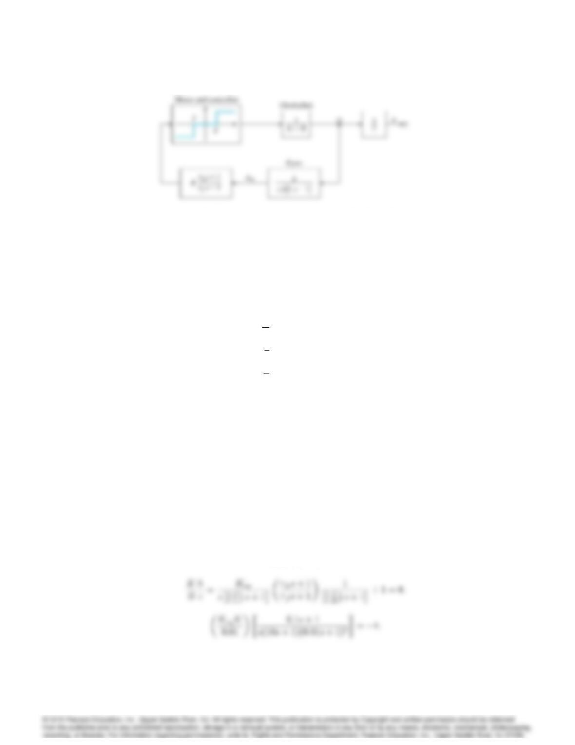
Figure 9.65: Block diagram of the system for Problem 9.15.

Problem 9.14. DF values for several di¤erent input frequencies.

15. A contactor controller of an inertial platform is shown in Figure 9.65 where

I= 0:1kgm2

I

B= 10 sec

h

c= 1

J

c= 0:01 sec

L= 0:1 sec

f= 0:01 sec

d= 105rad

T= 1Nm

The required stabilization resolution is approximately 106rad

K‘m> d for ‘m>106rad

Discuss the existence, amplitude and frequency of possible limit cycles as a function of the gain

Kand the DF of the controller. Repeat the problem for a deadband with hysteresis.

Solution: Limit cycles depend on the natural behavior of the closed-loop part. The DF of the

switch =Keq:Characteristic equation is:

KG + 1 = 0

9024 CHAPTER 9. NONLINEAR SYSTEMS

–150

–50

0

Magnitude (dB)

10

-3

10

-2

10

-1

10

0

10

1

10

2

10

3

–225

–135

Freq uency (rad/sec)

–150

–50

0

Magnitude (dB)

10

-3

10

-2

10

-1

10

0

10

1

10

2

10

3

–225

–135

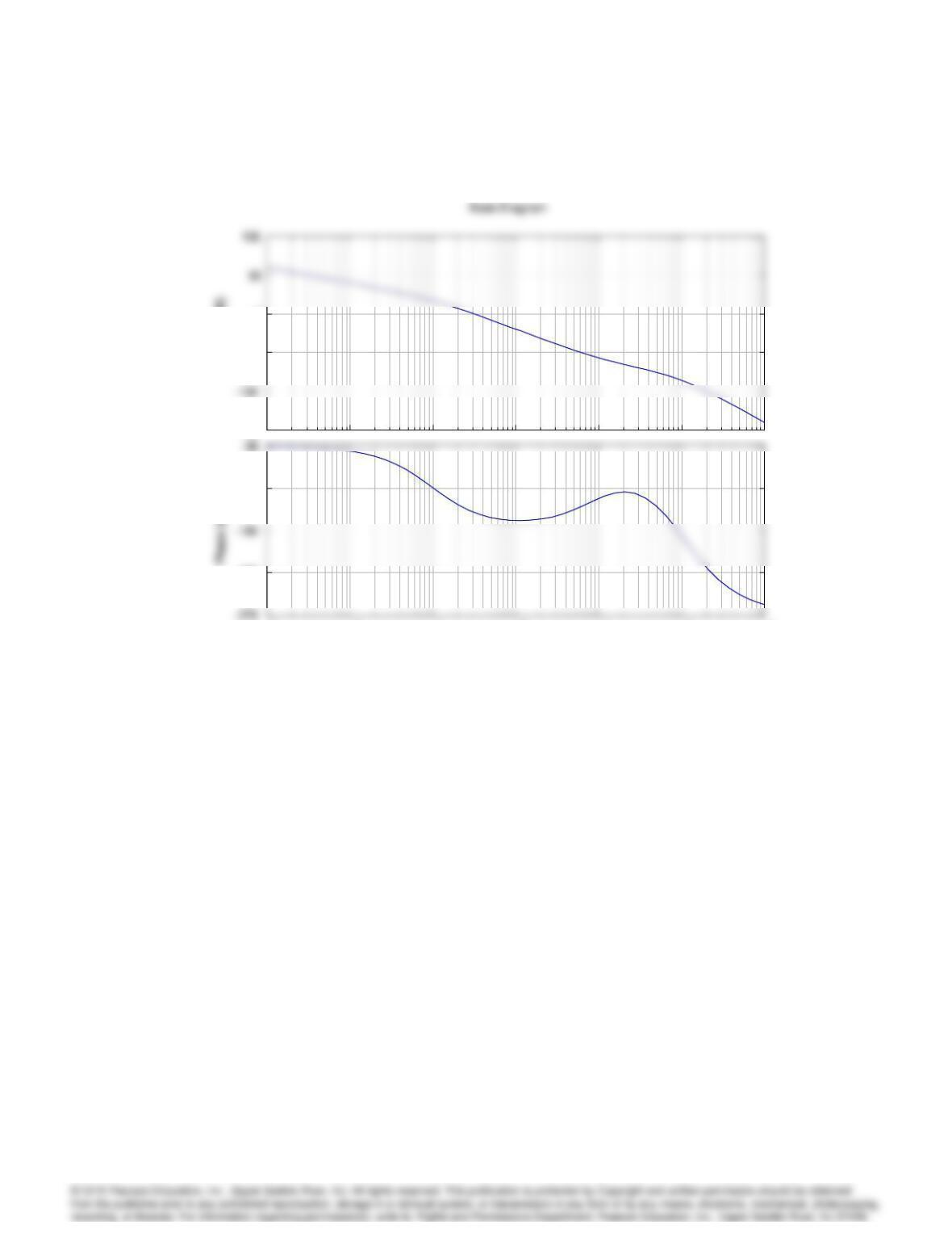
Frequency response for Problem 9.15.

9025

–150 – 100 –50 050

–50

Root Locus

Real Axis

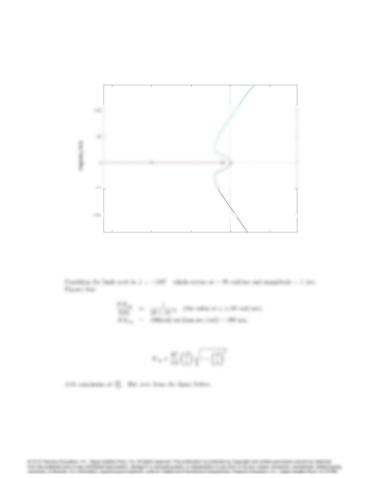
Root locus for Problem 9.15.

Fig

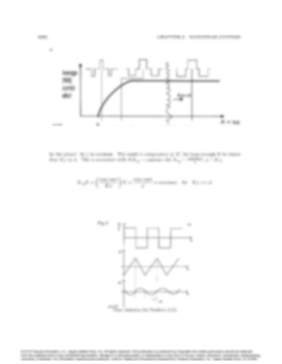
Response for nonlinear system for Problem 9.15.

that for levels of say a > 3d, the output is a constant. The frequency of the limit cycle is fixed

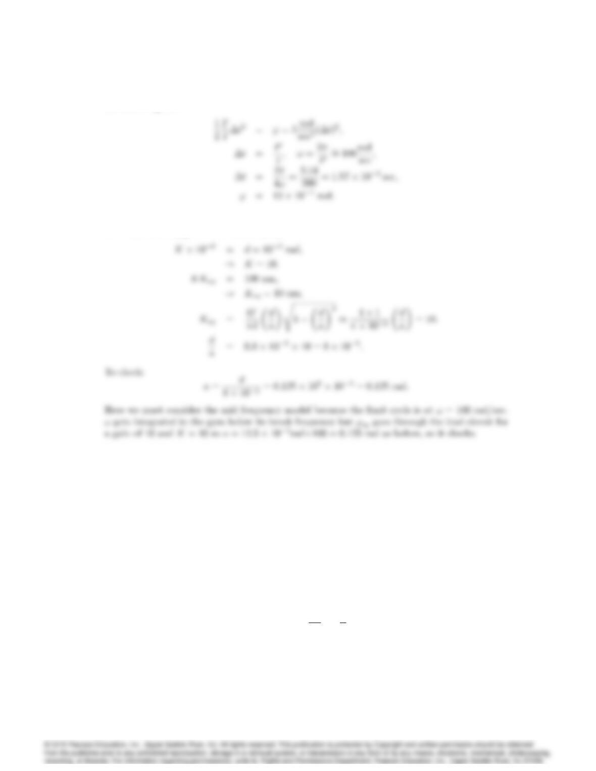
The amplitude is:

9027

See above figures:

If the resolution of platform picko¤ should be 106rad and “short” term sensor noise 

106rad, then K‘m>> d is satisfied, say,

16. Nonlinear Clegg Integrator There have been some attempts over the years to improve upon the

linear integrator. A linear integrator has the disadvantage of having a phase lag of 90at all

frequencies. In 1958, J. C. Clegg suggested that we modify the linear integrator to reset its

state, x, to zero whenever the input to the integrator, e, crosses zero (i.e., changes sign). The

Clegg integrator has the property that it acts like a linear integrator whenever its input and

output have the same sign. Otherwise, it resets it output to zero. The Clegg integrator can

be described by

x(t) = e(t)if e(t)6= 0;

x(t+) = 0 if e(t) = 0;

where the latter equation implies that the state of the integrator, x, is reset to zero immediately

after echanges sign. The Clegg integrator can be implemented with op-amps and diodes. A

potential disadvantage of the Clegg integrator is that it may induce oscillations. (a) Sketch the

output of the Clegg integrator if the input is e=asin(!t). (b) Prove that the DF for the Clegg

integrator is

N(a; !) = 4

! j1

!:

and this amounts to a phase lag of only 38.

Solution: (a) See Figure below.

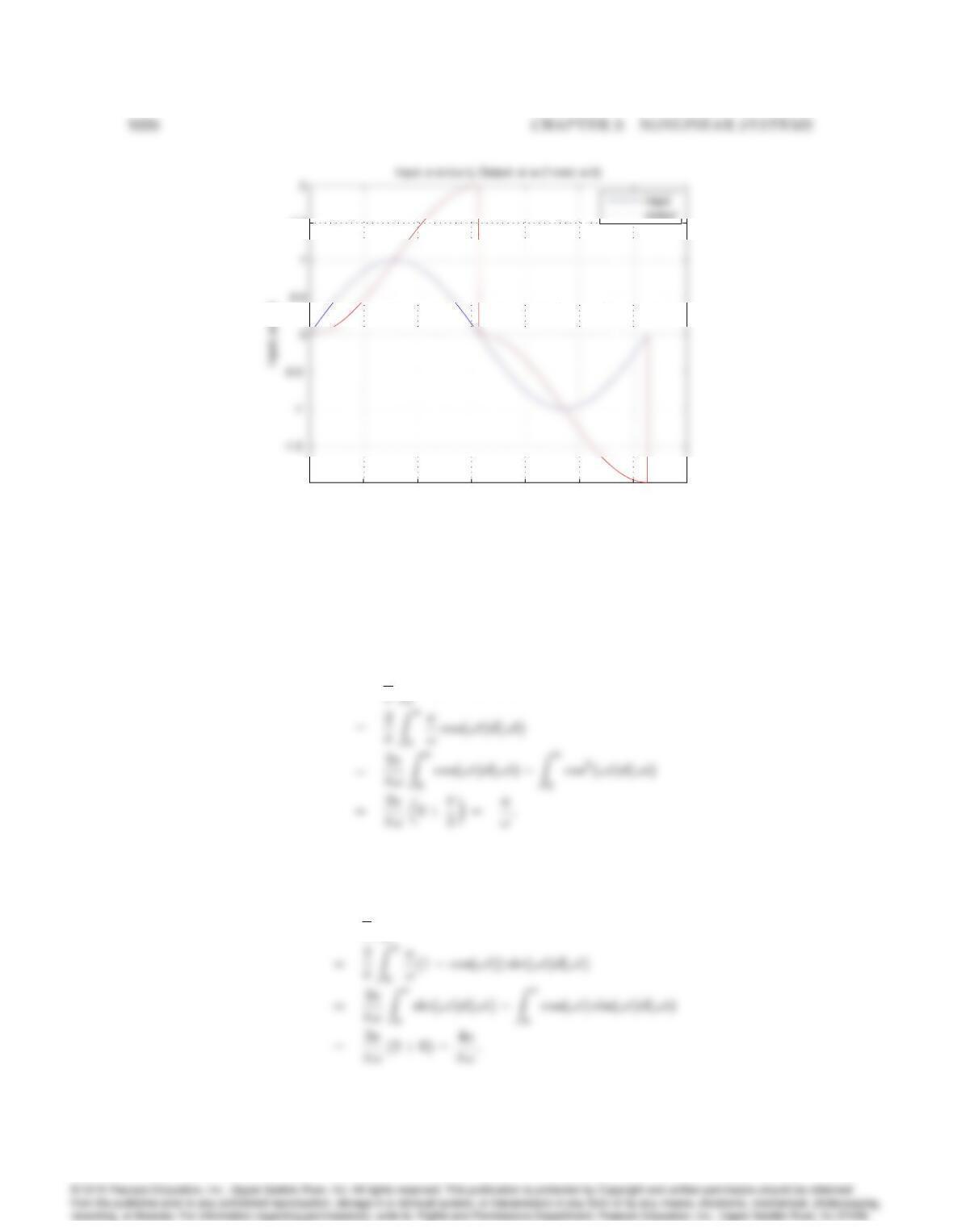
0 1 2 3 4 5 6 7

-2

1.5

ω t

Plots of the input and output signals.

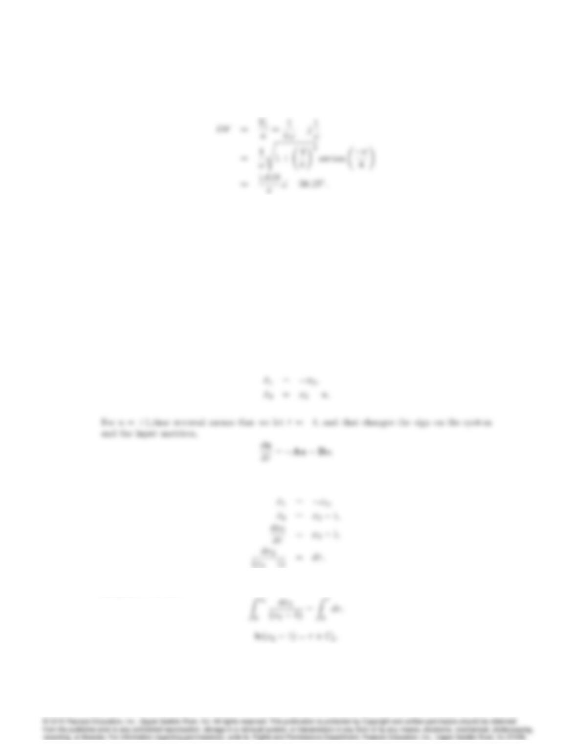
(b)

a1=2

x(t) cos(!t)d(!t)

b1=2

Z

0

x(t) sin(!t)d(!t)

9029

The describing function is then given by,

Problems and Solutions for Section 9.5: Analysis and De–

sign Based on Stability

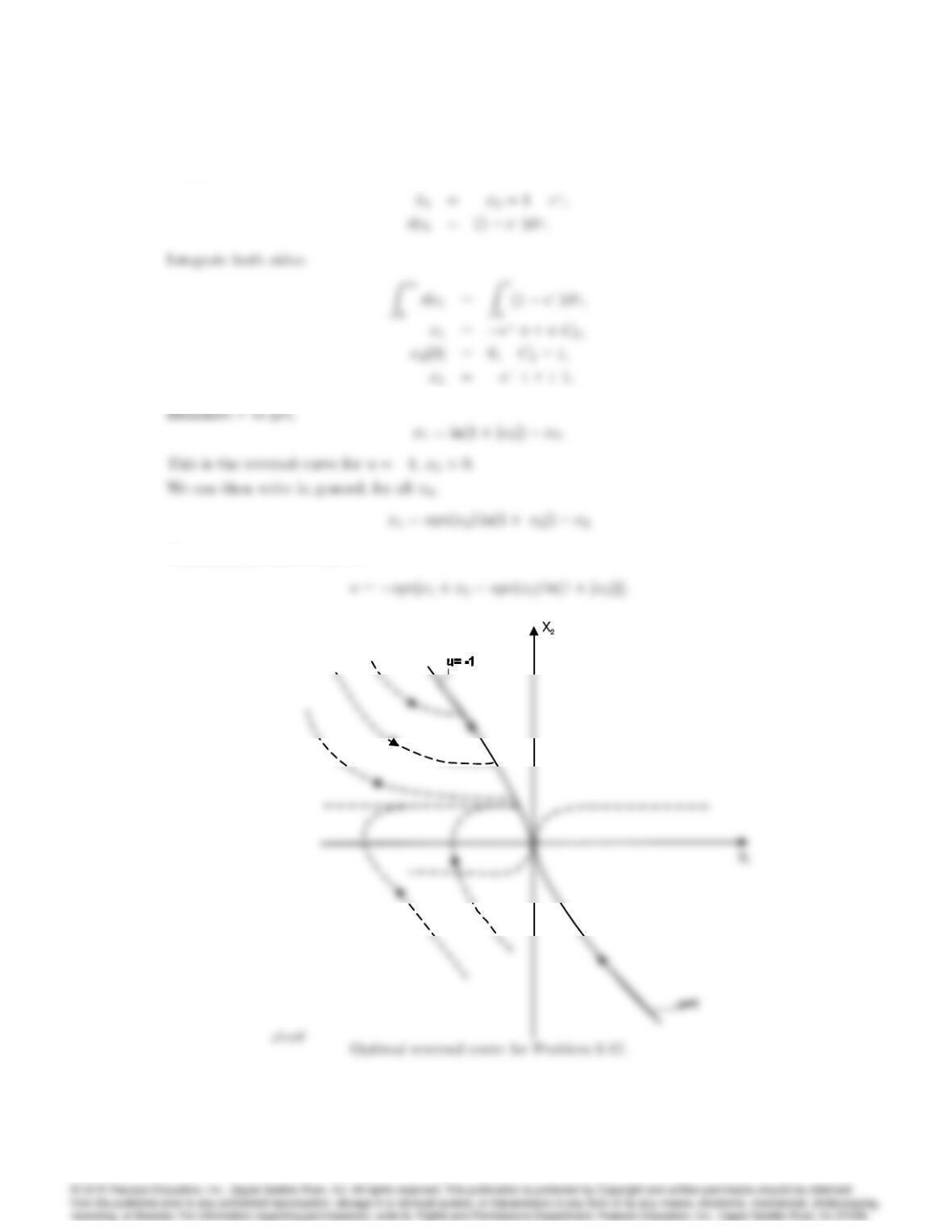
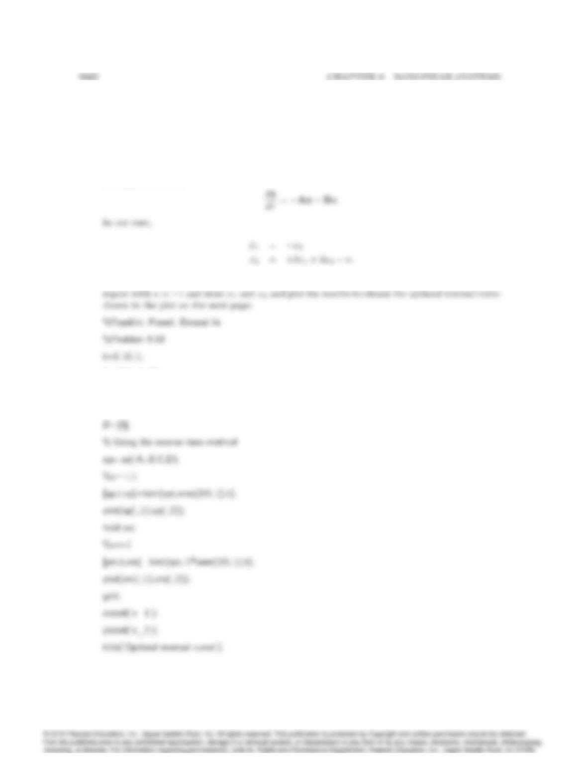
17. Compute and sketch the optimal reversal curve and optimal control for the minimal time control

of the plant

_x1=x2

_x2=x2+u

juj  1

Use the reverse time method and eliminate the time.

Solution: Use the reverse time method and eliminate the time:

In our case,

Integrate both sides: Zx2

9030 CHAPTER 9. NONLINEAR SYSTEMS

Since x2(0) = 0 then,

Now,

Integrate both sides:

Eliminate to get,

Integrate both sides:

9031

Now,

Therefore, the control law is:

Fig 14

18. Sketch the optimal reversal curve for the minimal time control with juj  1of the linear plant

_x1=x2

_x2=2x13x2+u:

Solution: We reverse time that means =t, and that changes the sign on the system and

the input matrices,

We simulate the system using the Matlab lsim function with u= +1 and store x1and x2, and

A=[0 1;-2 -3];

B=[0;1];

C=[1 0];

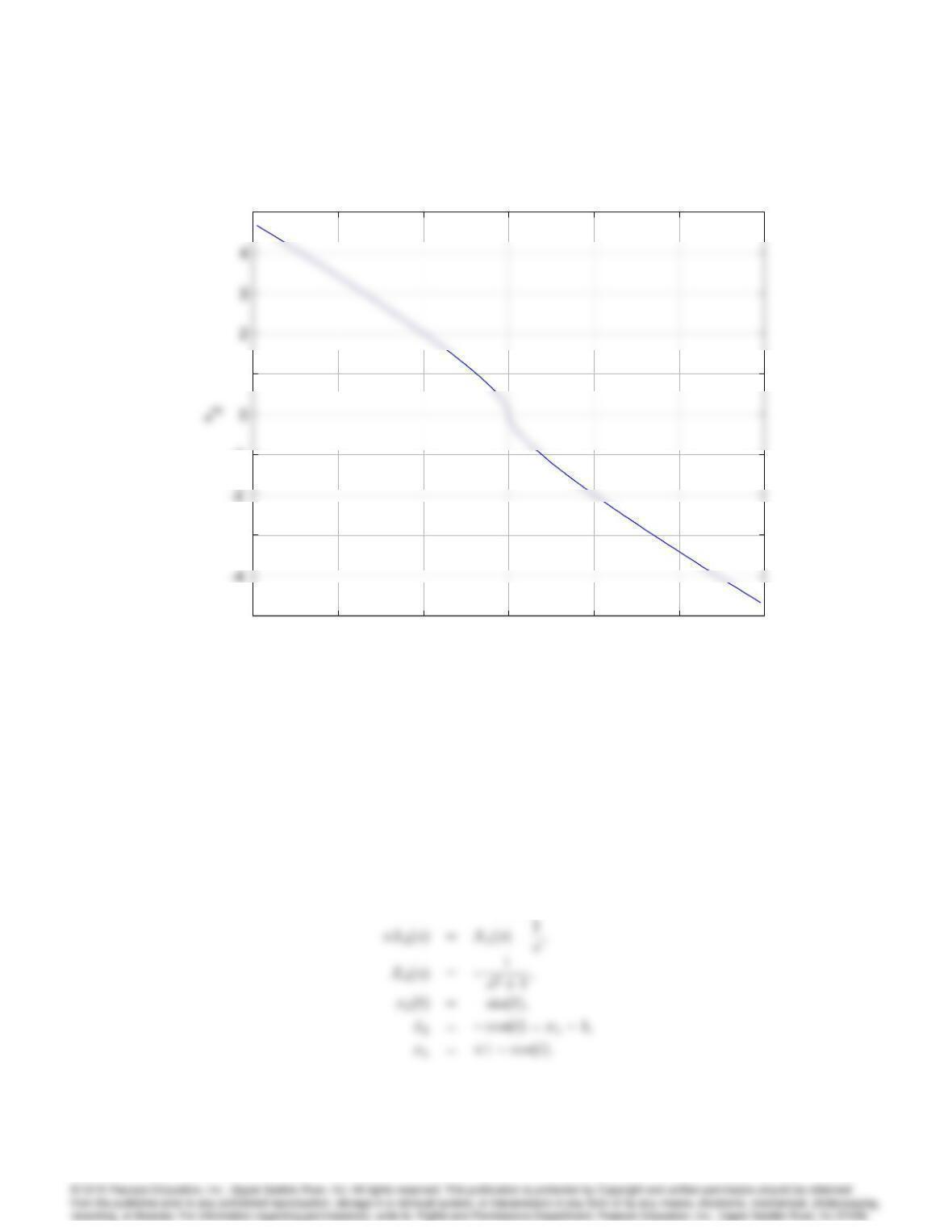
9033

–1.5 -1 –0.5 00.5 11.5

-5

-3

-1

1

5

x1

Optimal reversal curve

–1.5 -1 –0.5 00.5 11.5

-5

-3

-1

1

5

x1

Optimal reversal curve

Optimal reversal curve for Problem 9.18.

19. Sketch the time optimal control law for

_x1=x2

_x2=x1+u

juj  1

and show a trajectory for x1(0) = 3, and x2(0) = 0.

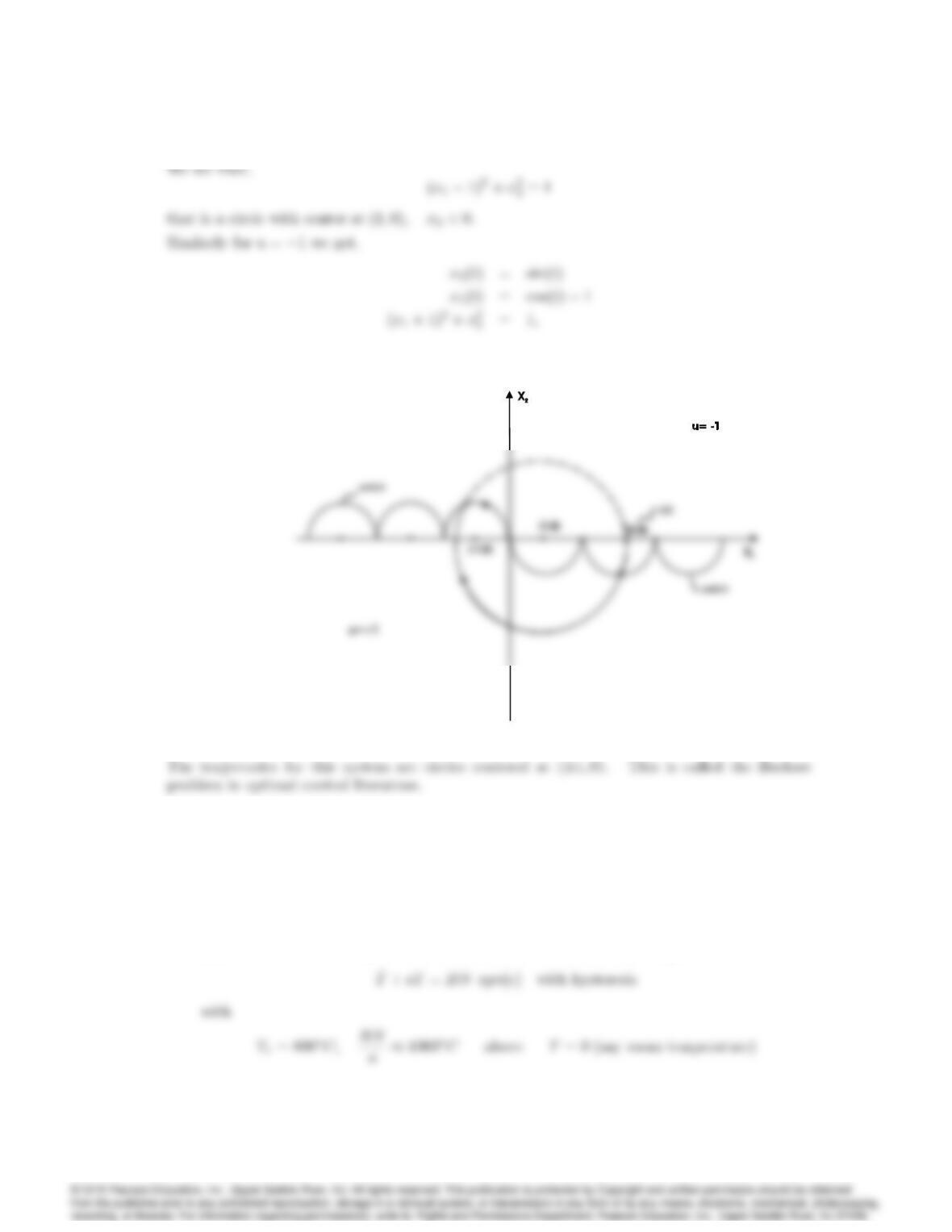
Solution: u= +1,

sX1(s) = X2(s);

9034 CHAPTER 9. NONLINEAR SYSTEMS

that is a circle with center at (1;0); x2>0:

Fig 12

30:pdf

Reversal curves for Problem 9.19.

20. Consider the thermal control system shown in Figure 9.66. The physical plant can be a room,

an oven, etc.

(a) What is the limit cycle period?

(b) If Tris commanded as a slowly increasing function, sketch the output of the system, T.

Show the solution for Tr“large”.

Solution:

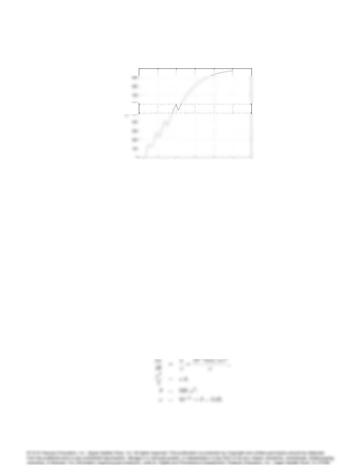
(a) This is a first order system so use (T; t) plot. For an oven, it is piecewise linear

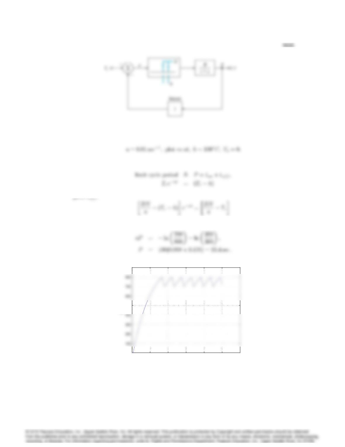
Figure 9.66: Thermal system for Problem 9.20

(b)

gives ton,

0 1 2 3 4 5 6

x 104

0

500

900

T ime (sec)

Temperature output for Problem 9.20.

(c) See Figure below.

9036 CHAPTER 9. NONLINEAR SYSTEMS

0 1 2 3 4 5 6

x 104

0

600

1000

T ime (sec

Temperature output for reference input Tr= 3tfor Problem 9.20.

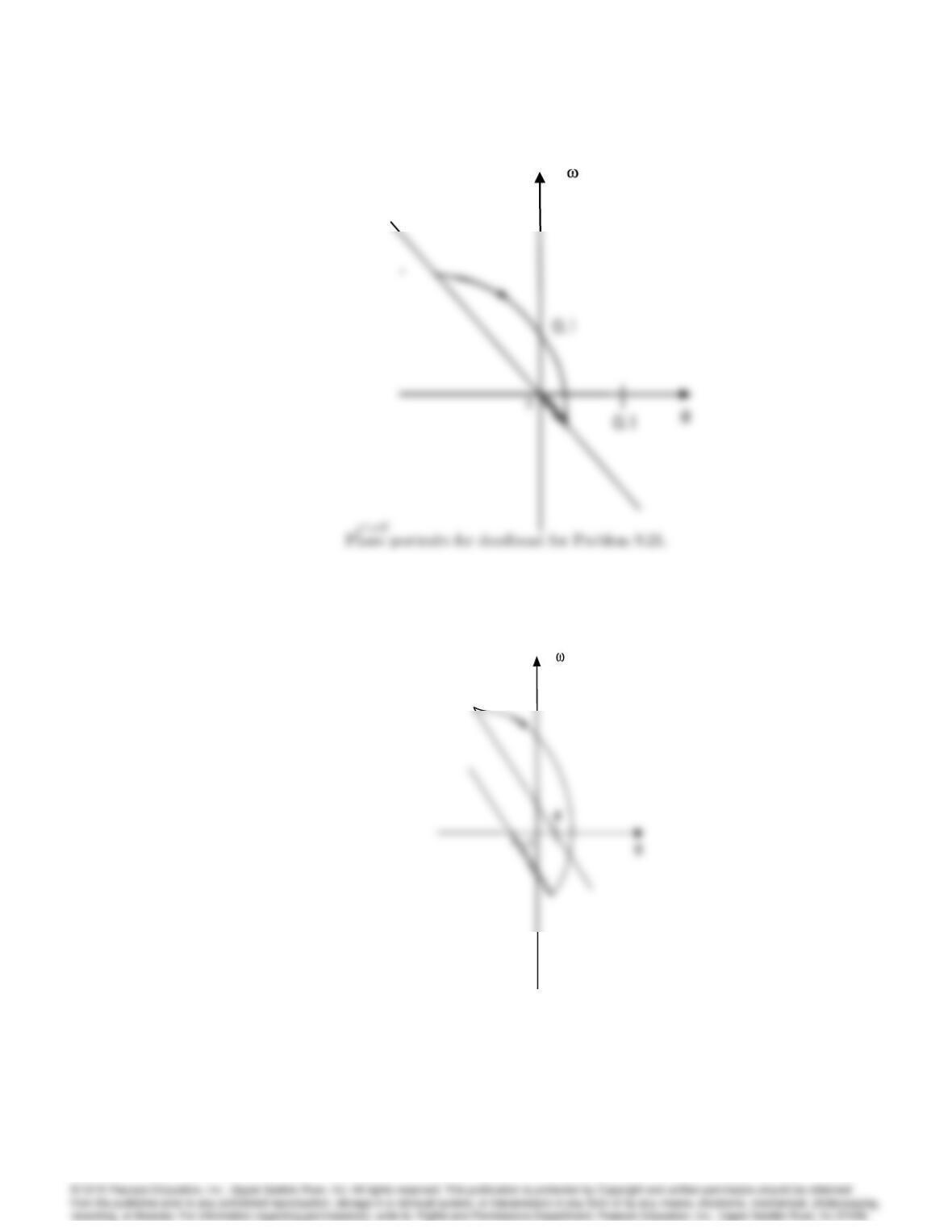
21. Several systems such as spacecraft, spring-mass system with resonant frequency well below the

frequency of switching, a large motor driven load with very small friction, etc. can be modeled

as just an inertia. For an ideal switching curve, sketch the phase portraits of the system. The

switching function is e=+!. Assume = 10 sec, and the control signal = 103rad/sec2.

Now sketch the results with,

a) deadband,

b) deadband plus hysteresis,

c) deadband plus time delay T,

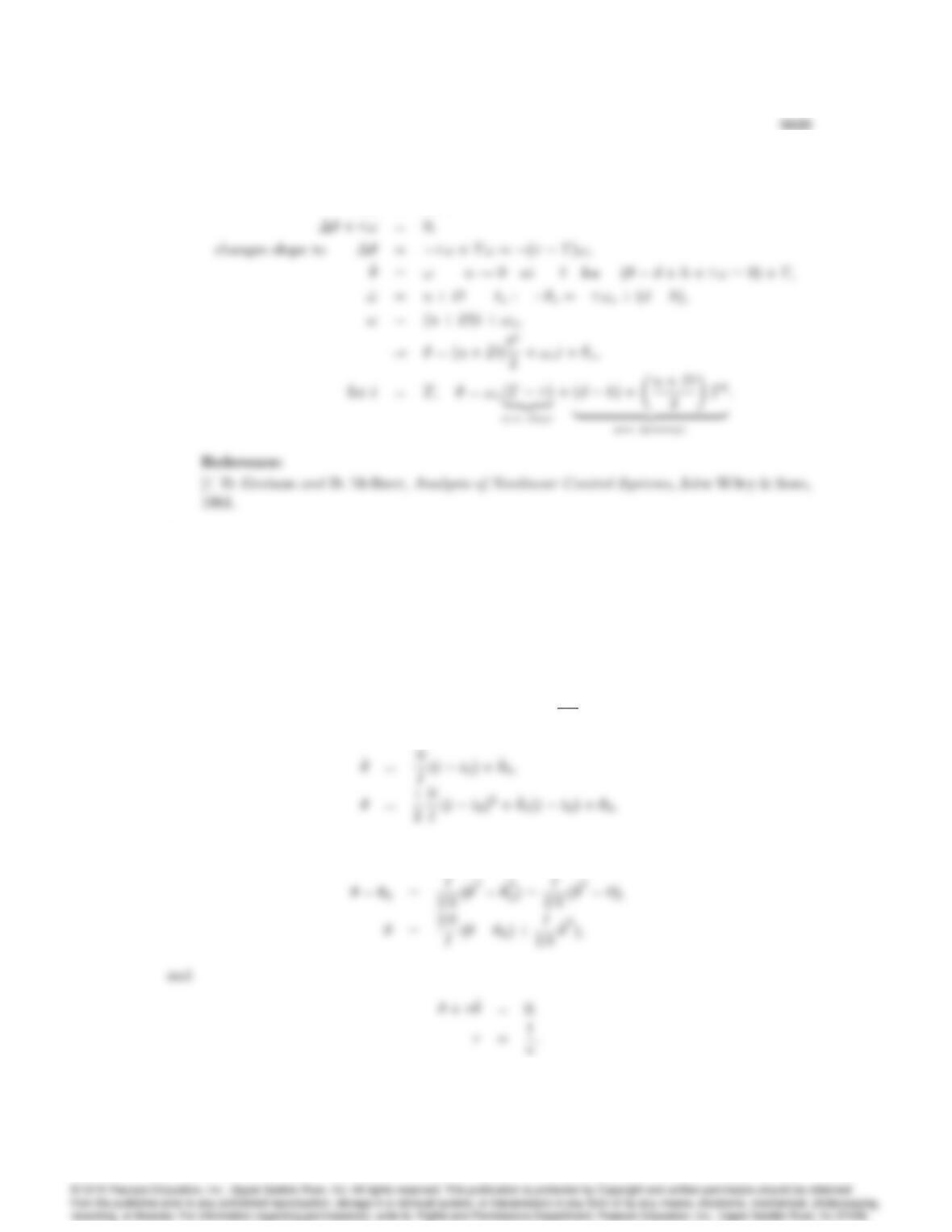
d) deadband plus a constant disturbance.

Solution:

(a)

9037

Fig 1

(a)

Fig 2

35:pdf

Phase portraits for deadband for Problem 9.21.

(b)

9038 CHAPTER 9. NONLINEAR SYSTEMS

Fig 3

36:pdf

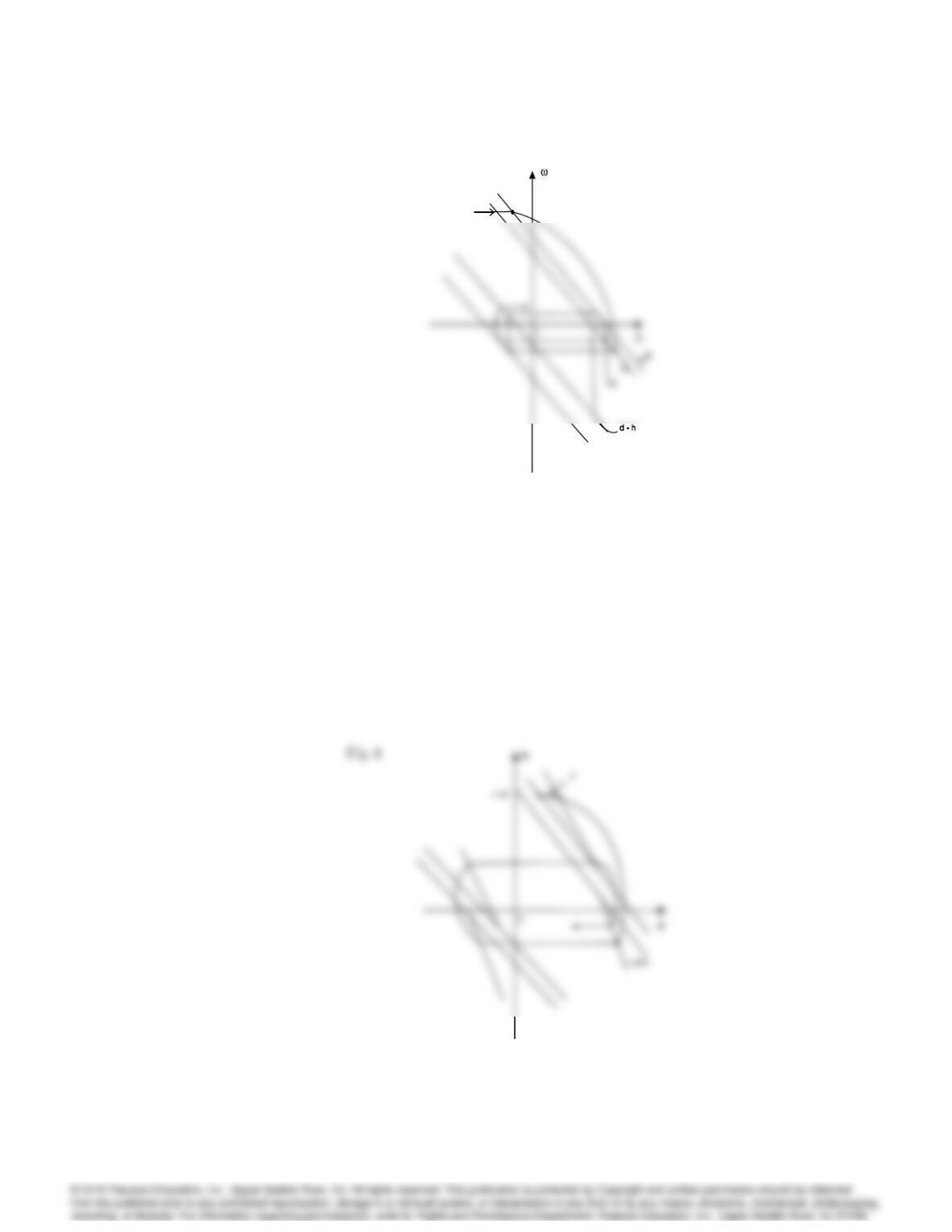
Phase portraits for deadband plus hysteresis for Problem 9.21.

(c)

37:pdf

Phase portraits for deadband plus plus time delay Tfor Problem 9.21.

(d)

T ! = ;

22. Compute the amplitude of the limit cycle in the case of satellite attitude control with delay

I•

=N u(t)

using

u=sgn(_

+)

Sketch the phase plane trajectory of the limit cycle and time history of giving the maximum

value of .

Solution: Since the delay is seconds, _

must travel N

Iunits during the delay. We can

obtain the following relations:

Eliminating (tt0), we get