Operating Systems Chapter 8 Homework Discretize The Pid Controller Using A Tustins

8000

Solutions Manual: Chapter 8

7th Edition

Feedback Control of Dynamic

Systems

Gene F. Franklin

.J. David Powell

.Abbas Emami-Naeini

Assisted by:

H. K. Aghajan

H. Al-Rahmani

P. Coulot

P. Dankoski

S. Everett

R. Fuller

T. Iwata

V. Jones

F. Safai

L. Kobayashi

H-T. Lee

E. Thuriyasena

M. Matsuoka

Chapter 8

Digital Control

Problems and Solutions for Section 8.2: Dynamic

Analysis of Discrete Systems

1. The z-transform of a discrete-time filter h(k)at a 1Hz sample rate is

H(z) = 1 + (1=2)z1

[1 (1=2)z1][1 + (1=3)z1]:

(a) Let u(k)and y(k)be the discrete input and output of this filter. Find

a difference equation relating u(k)and y(k).

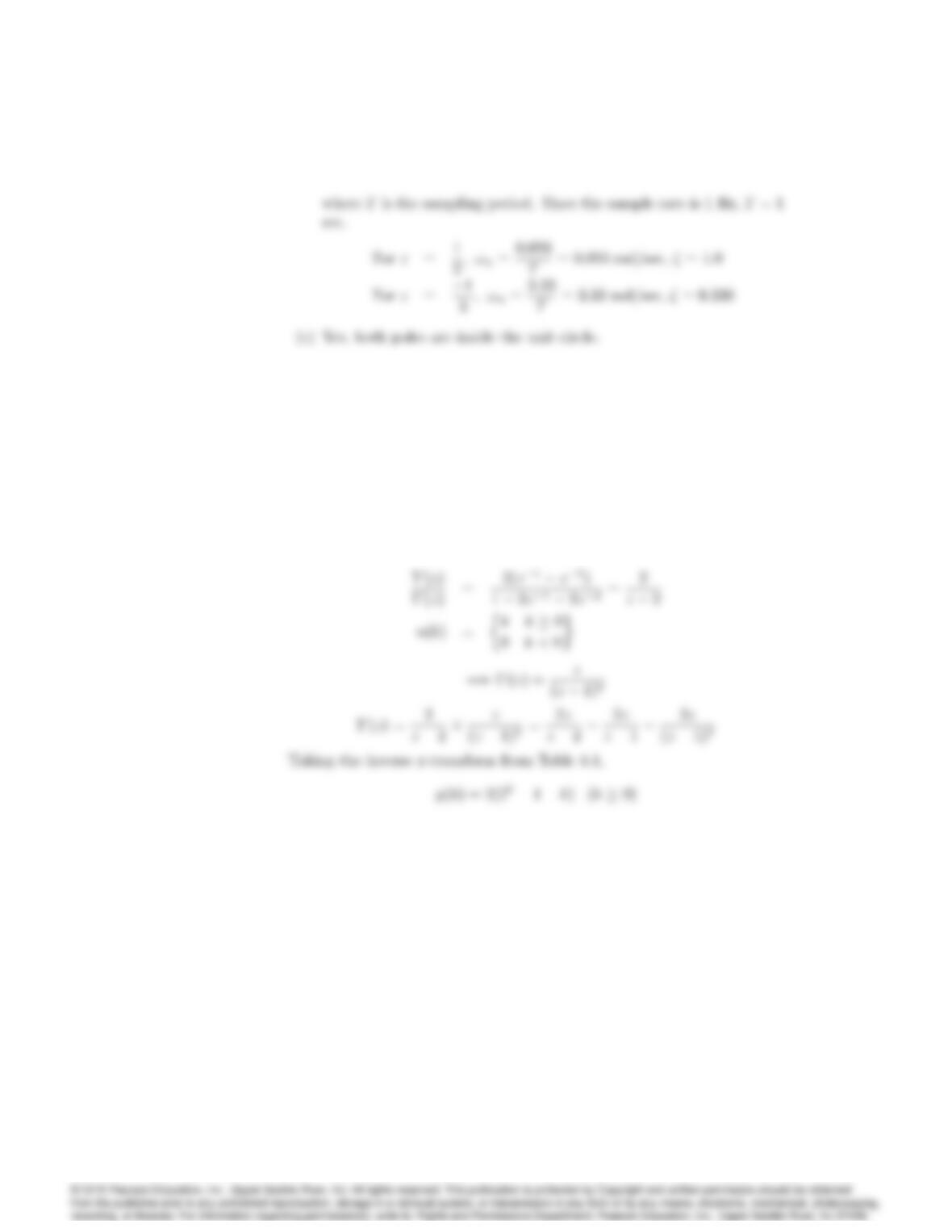
(b) Find the natural frequency and damping coefficient of the filter’s

poles

(c) Is the filter stable?

Solution:

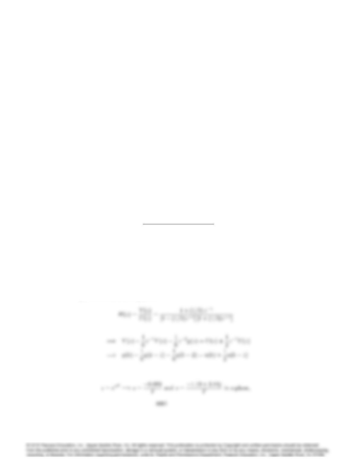
(a) Find a difference equation :

(b) Two poles at z= 1=2and z=1=3in z-plane.

8002 CHAPTER 8. DIGITAL CONTROL

2. Use the z-transform to solve the difference equation

y(k)3y(k1) + 2y(k2) = 2u(k1) 2u(k2);

where

u(k) = k; k 0;

0; k < 0;

y(k) = 0; k < 0:

Solution:

3. The one-sided z-transform is defined as

F(z) = 1

X

0

f(k)zk:

(a) Show that the one-sided transform of f(k+ 1) is Zff(k+ 1)g=

zF (z)zf(0).

(b) Use the one-sided transform to solve for the transforms of the Fi-

bonacci numbers generated by the difference equation u(k+ 2) =

u(k+ 1) + u(k). Let u(0) = u(1) = 1. [Hint: You will need to find

a general expression for the transform of f(k+ 2) in terms of the

transform of f(k)].

8003

(c) Compute the pole locations of the transform of the Fibonacci num-

bers.

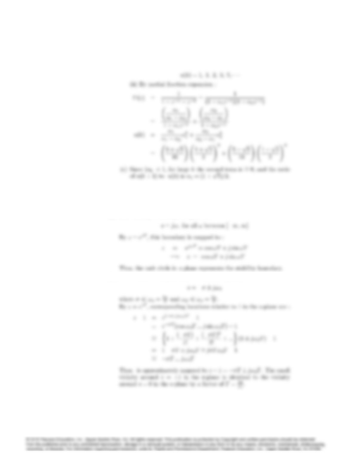
(d) Compute the inverse transform of the Fibonacci numbers.

(e) Show that, if u(k)represents the kth Fibonacci number, then the

ratio u(k+ 1)=u(k)will approach (1 + p5)=2. This is the golden

ratio valued so highly by the Greeks.

Solution:

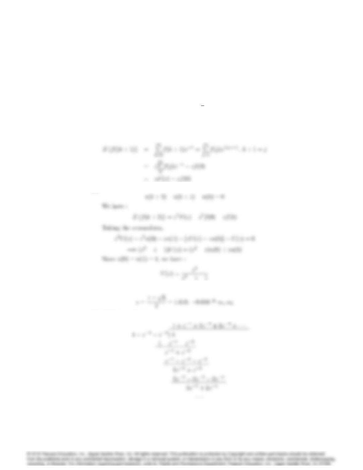
(a)

(b)

(c) The poles are at :

(d) (i) By long division :

8004 CHAPTER 8. DIGITAL CONTROL

4. Prove the seven properties of the s-plane-to-z-plane mapping listed in

Section 8.2.3.

Solution

(a) The stability boundary in s-plane is :

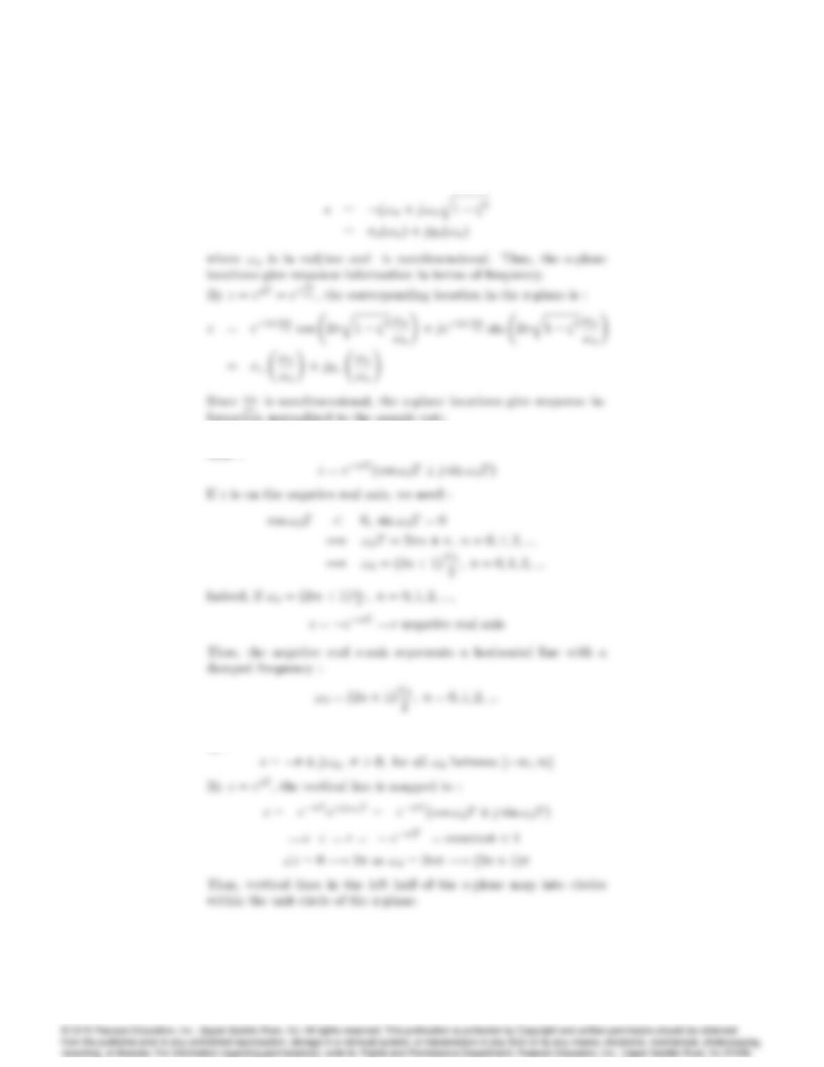
(b) In the small vicinity around s= 0 in the s-plane,

8005

(c) An arbitrary location in the s-plane is represented by :

formation normalized to the sample rate.

(d) Locations in the s-plane, s=j!d, are mapped to z-plane loca-

(e) An arbitrary vertical line in the left half of the s-plane is represented

by :

8006 CHAPTER 8. DIGITAL CONTROL

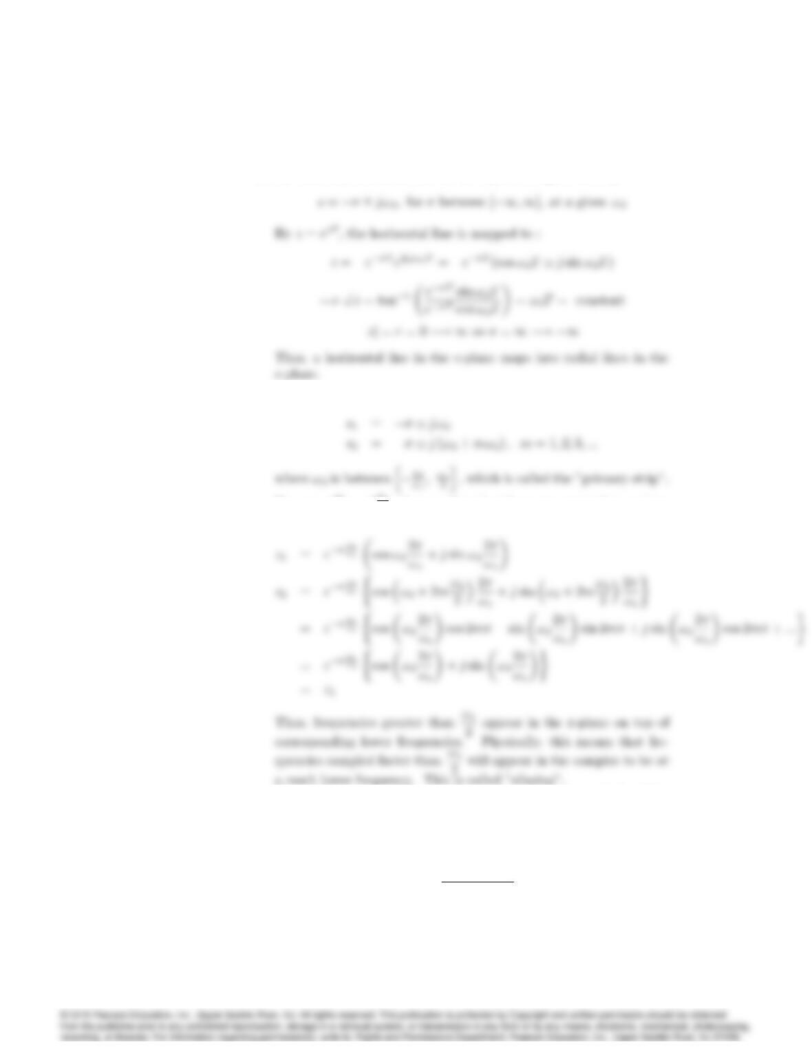
(f) An arbitrary horizontal line in the s-plane is represented by :

(g) Let s-plane locations s1and s2be :

By z=esT =es2

!s, these s-plane locations are mapped to z-plane

locations :

Problems and Solutions for Section 8.3: De–

sign using Discrete Equivalents

5. A unity feedback system has an open-loop transfer function given by

G(s) = 250

s[(s=10) + 1]:

8007

The following lag compensator added in series with the plant yields a

phase margin of 50:

Dc(s) = s=1:25 + 1

50s+ 1 :

Using the matched pole-zero approximation, determine an equivalent dig-

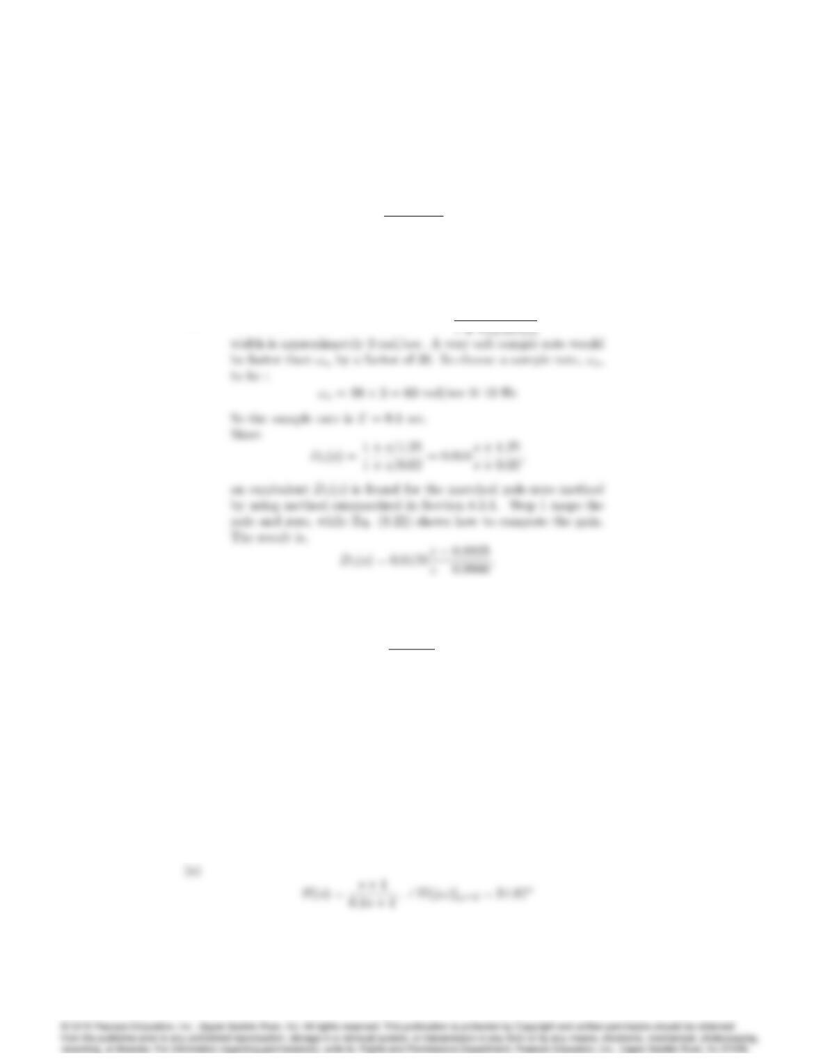
ital realization of this compensator.

Solution:

(a) For the compensated closed-loop system, Dc(s)G(s)

6. The following transfer function is a lead network designed to add about

60of phase at !1= 3 rad=sec:

H(s) = s+ 1

0:1s+ 1:

(a) Assume a sampling period of T= 0:25 sec, and compute and plot

in the z-plane the pole and zero locations of the digital implementa-

tions of H(s)obtained using (1) Tustin’s method and (2) pole-zero

mapping. For each case, compute the amount of phase lead provided

by the network at z1=ej!1T

(b) Using a log-log scale for the frequency range != 0:1to != 100 rad/sec,

plot the magnitude Bode plots for each of the equivalent digital sys-

tems you found in part (a), and compare with H(s). (Hint: Magni-

tude Bode plots are given by jH(z)j=jH(ej!T )j.)

Solution:

8008 CHAPTER 8. DIGITAL CONTROL

(1) Tustin’s method, analytically :

or, via Matlab:

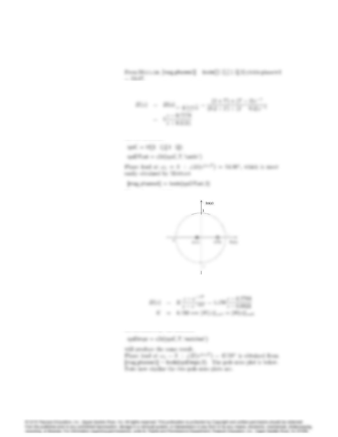
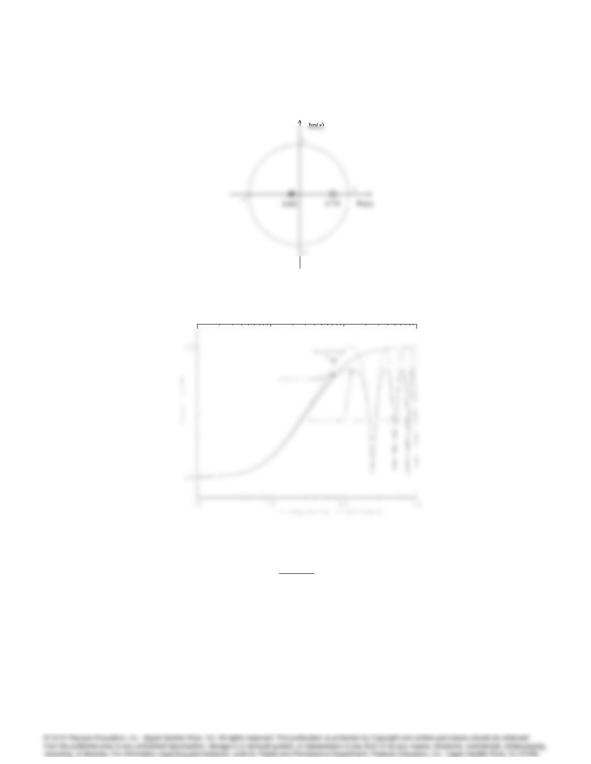
The pole-zero plot is:

(2) Matched pole-zero method, analytically :

or, alternatively via Matlab

8009

(b) The Bode plots match fairly well until the frequency approaches

the half sample frequency (

=12 rad/sec), at which time the

curves diverge.

7. The following transfer function is a lag network designed to introduce a

gain attenuation of 10(20dB) at !1= 3 rad/sec:

H(s) = 10s+ 1

100s+ 1:

(a) Assume a sampling period of T= 0:25 sec, and compute and plot

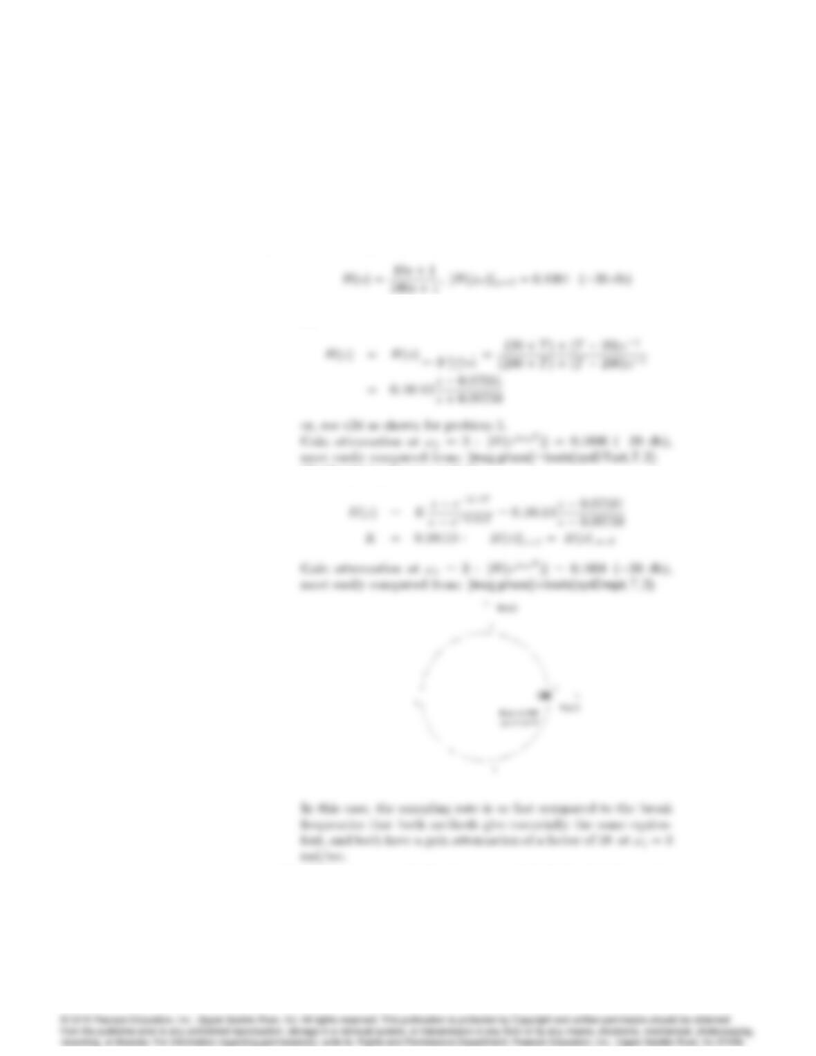
in the z-plane the pole and zero locations of the digital implementa-

tions of H(s)obtained using (1) Tustin’s method and (2) pole-zero

mapping. For each case, compute the amount of gain attenuation

provided by the network at z1=ej!1T.

8010 CHAPTER 8. DIGITAL CONTROL

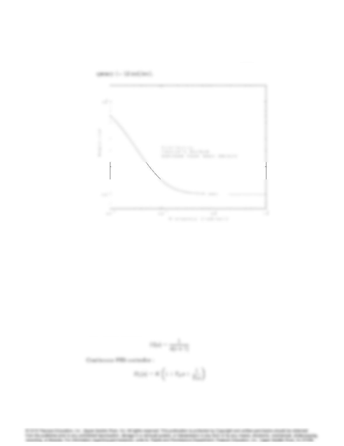
(b) For each of the equivalent digital systems in part (a), plot the Bode

magnitude curves over the frequency range != 0:01 to 10 rad/sec.

Solution:

(a) First, we’ll compute the attenuation of the continuous system,

(1) Tustin’s method :

(2) Matched pole-zero method :

(b) All three are essentially the same and indistinguishable on the

plot because the range of interest is below the half sample fre-

8011

Problems and Solutions for Section 8.5: Sam–

ple Rate Selection

8. For the system shown in Fig. 8.22, find values for K,TD, and TIso that

the closed-loop poles satisfy  > 0:5and !n>1rad/sec. Discretize

the PID controller using:

(a) Tustin’s method

(b) matched pole-zero method

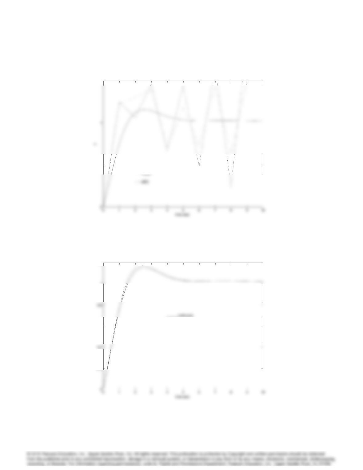
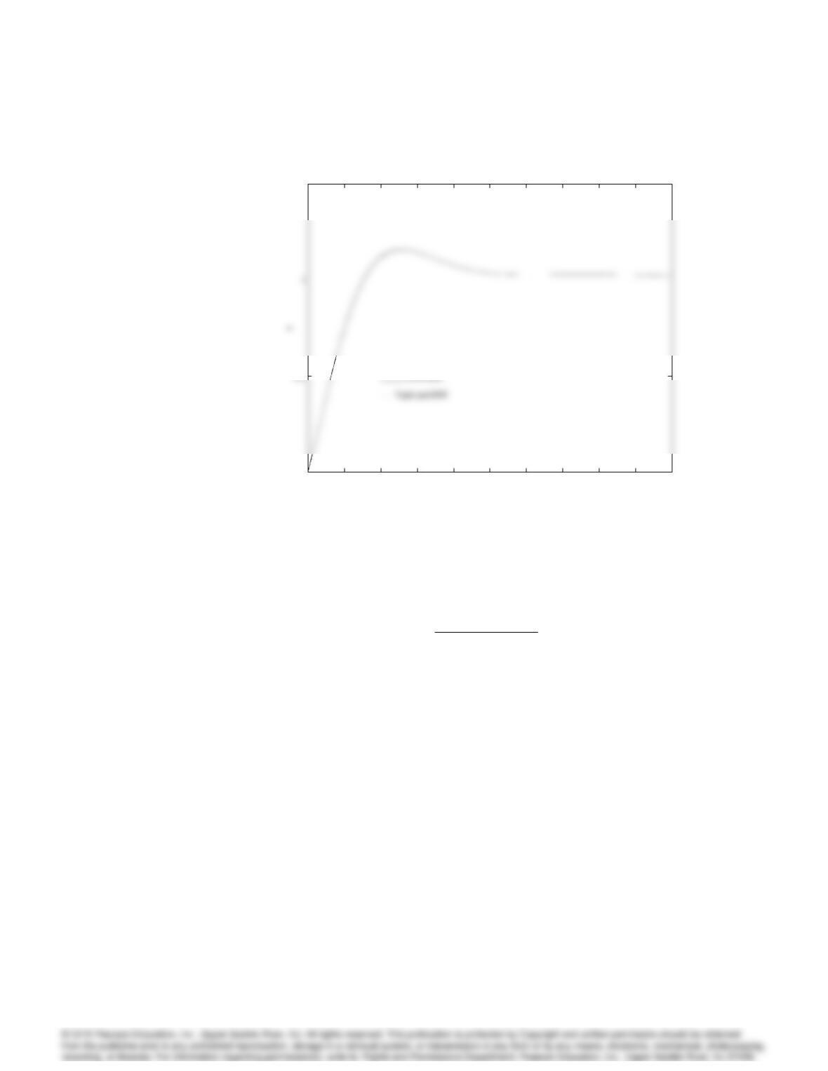
Use Matlab to simulate the step response of each of these digital imple-

mentations for sample times of T= 1, 0.1, and 0.01 sec.

Solution

(a) Continuous PID-controller design

Plant transfer function :

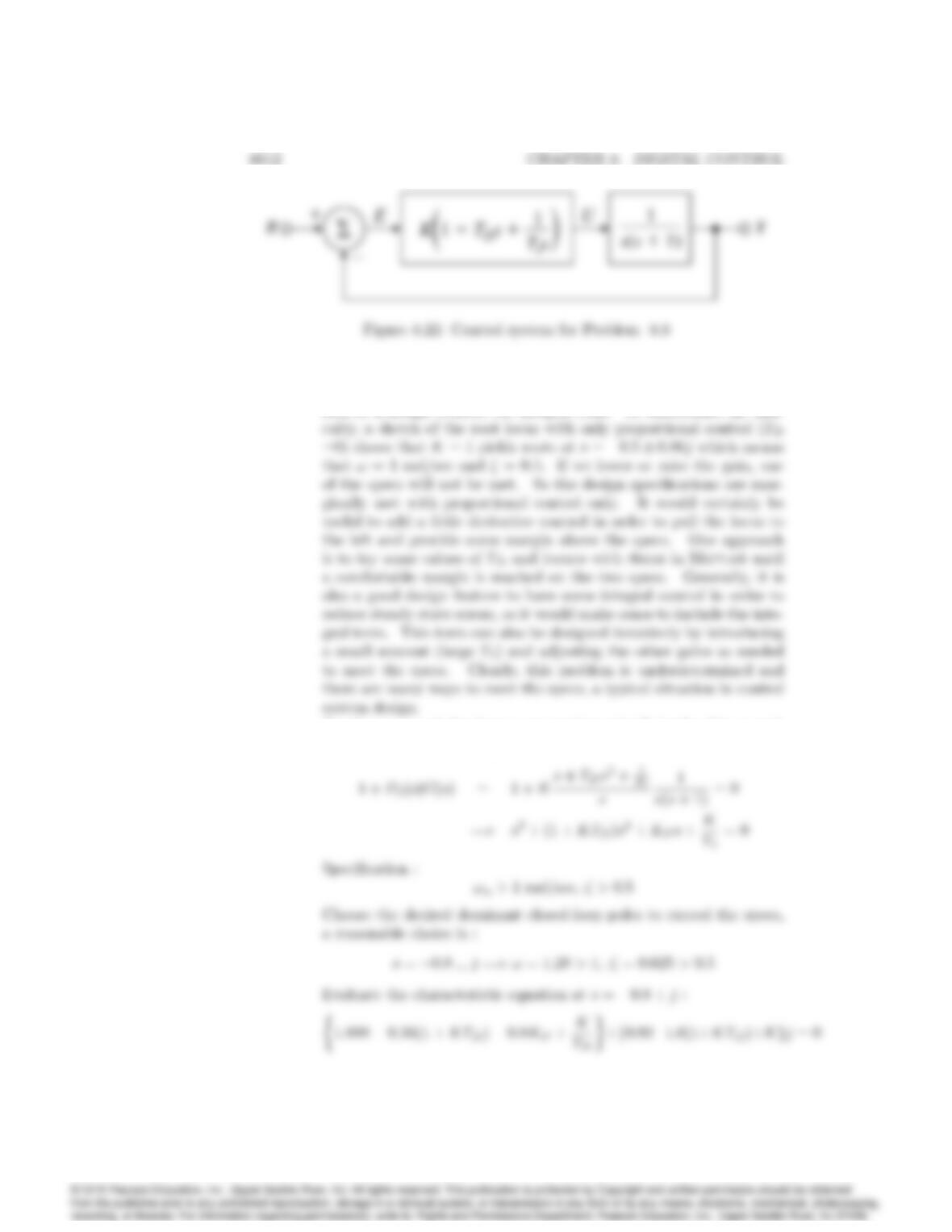
There is no requirement that there be an integral term, so first let’s

look at a design without the integral term. To understand the diffi-

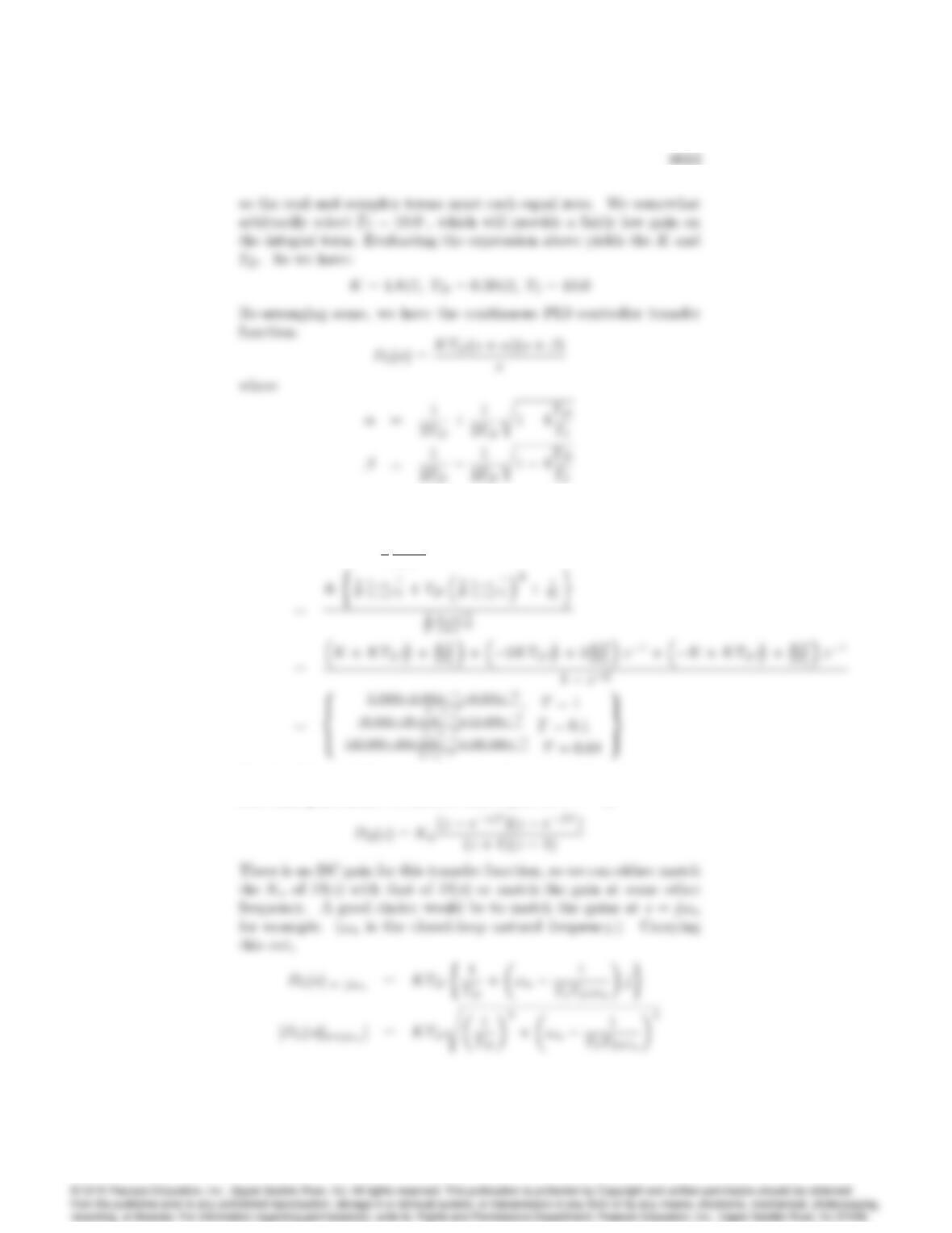
Another approach for those more mathematically inclined is to eval-

uate the characteristic equation :

(b) Discrete PID controller by Tustin’s method can be obtained analyt-

ically as below or by using c2d in Matlab :

Dd(z) = Dc(s)js=2

T

1z1

1+z1

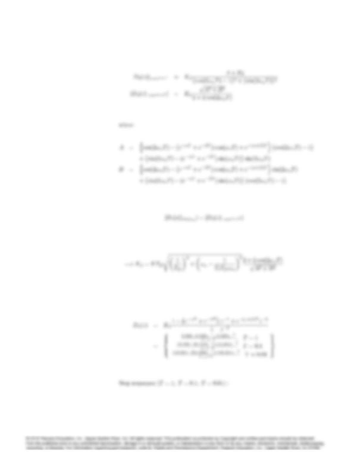
(c) For the Matched Pole-zero approximation, note there is one more

zero than pole, hence we need to add a pole at z=1,

8014 CHAPTER 8. DIGITAL CONTROL

Thus,

8015

0.5

1.5

Step Response (T=1)

____ Continuous

0.2

0.6

1

1.2

y

Step Response (T=0.1)

– – – tustin and MPZ

8016 CHAPTER 8. DIGITAL CONTROL

0 1 2 3 4 5 6 7 8 9 10

0

0.5

1.5

time (sec)

Step Response (T=0.01)

______ Continuous

Problems and Solutions for Section 8.6: Dis–

crete Design

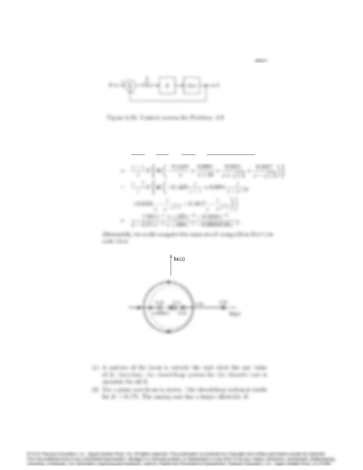
9. Consider the system configuration shown in Fig. 8.23, where

G(s) = 40(s+ 2)

(s+ 10)(s21:4):

(a) Find the transfer function G(z)for T= 1 assuming the system is

preceded by a ZOH.

(b) Use Matlab to draw the root locus of the system with respect to

K.

(c) What is the range of Kfor which the closed-loop system is stable?

(d) Compare your results of part (c) to the case where an analog con-

troller is used (that is, where the sampling switch is always closed).

Which system has a larger allowable value of K?

(e) Use Matlab to compute the step response of both the continuous

and discrete systems with Kchosen to yield a damping factor of

= 0:5for the continuous case.

Solution

(a) Using partial fraction expansion along with Table 8.1,

G(z) = z1

zZG(s)

s=z1

zZ40(s+ 2)

s(s+ 10)(s21:4)

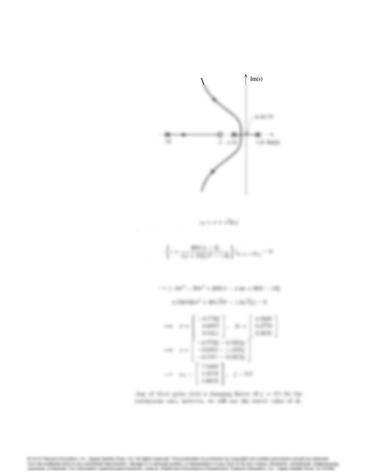
(b) The z-plane root locus is shown.

8018 CHAPTER 8. DIGITAL CONTROL

(e) Since = 0:5must be achieved, an analytical approach would

be to let a desired closed-loop pole be :

Evaluate the continuous characteristic equation at sd:

and find that a cubic results, i.e., there are three places on the

locus where = 0:5:

8019

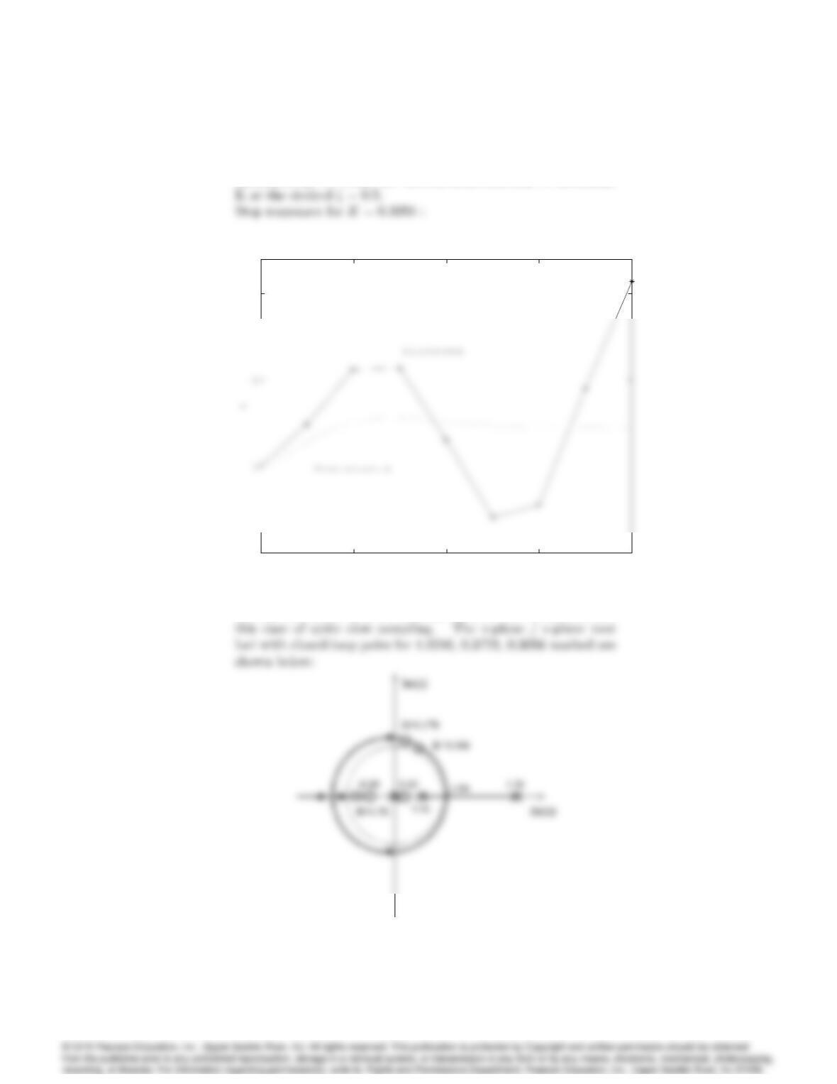
Alternatively, we could use rlocfind from Matlab to determine

0 2 4 6 8

-5

10

Closed-Loop Step Response (K=0.3056)

Time (sec)

As expected from the root loci, the discrete case is unstable for