Operating Systems Chapter 8 Homework Although Stated The Solution Problem 527 That

8020 CHAPTER 8. DIGITAL CONTROL

10. Single-axis Satellite Attitude Control: Satellites often require attitude con-

trol for proper orientation of antennas and sensors with respect to Earth.

Figure 2.7 shows a communication satellite with a three-axis attitude-

control system. To gain insight into the three-axis problem we often con-

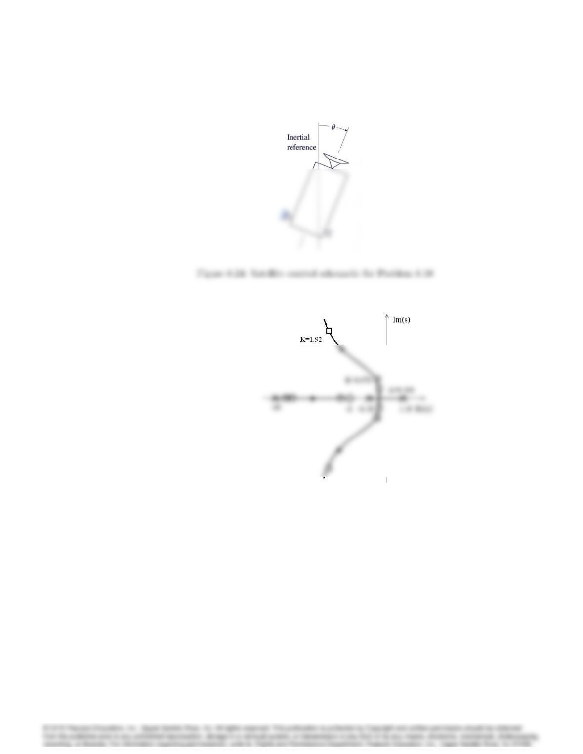
sider one axis at a time. Figure 8.24 depicts this case where motion is

only allowed about an axis perpendicular to the page. The equations of

motion of the system are given by

I•

=MC+MD;

where

8021

I = moment of inertia of the satellite about its mass center;

MC=control torque applied by the thrusters;

MD=disturbance torques;

=angle of the satellite axis with respect to an inertial reference with no

angular acceleration:

We normalize the equations of motion by defining

u=MC

I; wd=MD

I;

and obtain •

=u+wd:

Taking the Laplace transform yields

(s) = 1

s2[u(s) + wd(s)];

which with no disturbance becomes

(s)

u(s)=1

s2=G1(s):

In the discrete case where uis applied through a ZOH, we can use the

methods described in this chapter to obtain the discrete transfer function

G1(z) = (z)

u(z)=T2

2z+ 1

(z1)2:

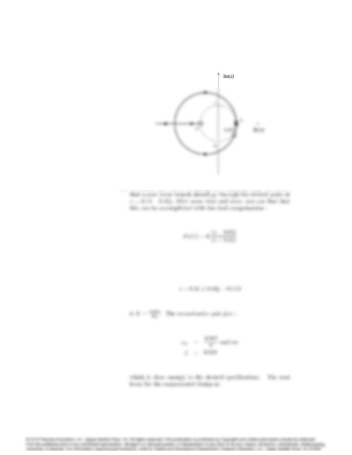
(a) Sketch the root locus of this system by hand assuming proportional

control.

(b) Draw the root locus using Matlab to verify the hand sketch.

(c) Add a discrete velocity feedback to your controller so that the dom-

inant poles correspond to = 0:5and !n= 3=(10T).

(d) What is the feedback gain if T= 1 sec? If T= 2 sec.

(e) Plot the closed-loop step response and the associated control time

history for T= 1 sec.

Solution

(a) The hand sketch will show that the loci branches depart vertically

8022 CHAPTER 8. DIGITAL CONTROL

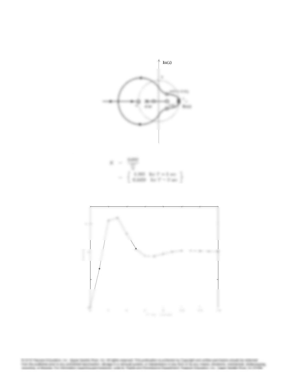
(c) To obtain the desired damping and frequency, Fig. 8.4 shows

The specific value of Kthat yields the closed-loop poles are at :

8023

(d)

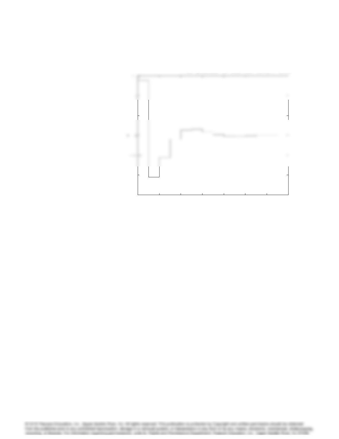
(e) Closed-loop step response :

0.5

Closed-Loop Step Response (T=1s)

8024 CHAPTER 8. DIGITAL CONTROL

0 2 4 6 8 10 12 14

-1.5

-1

0.5

Time (sec)

11. It is possible to suspend a mass of magnetic material by means of an

electromagnet whose current is controlled by the position of the mass

(Woodson and Melcher, 1968). The schematic of a possible setup is shown

in Fig. 8.25, and a photo of a working system at Stanford University is

shown in Fig. 9.2. The equations of motion are

m•x=mg +f(x; I);

where the force on the ball due to the electromagnet is given by f(x; I).

At equilibrium the magnet force balances the gravity force. Suppose we

let I0represent the current at equilibrium. If we write I=I0+i, expand

fabout x= 0 and I=I0, and neglect higher-order terms, we obtain the

linearized equation

m•x=k1x+k2i: (1)

Reasonable values for the constants in Eq. (1) are m= 0:02 kg,k1= 20

N=m, and k2= 0:4 N=A.

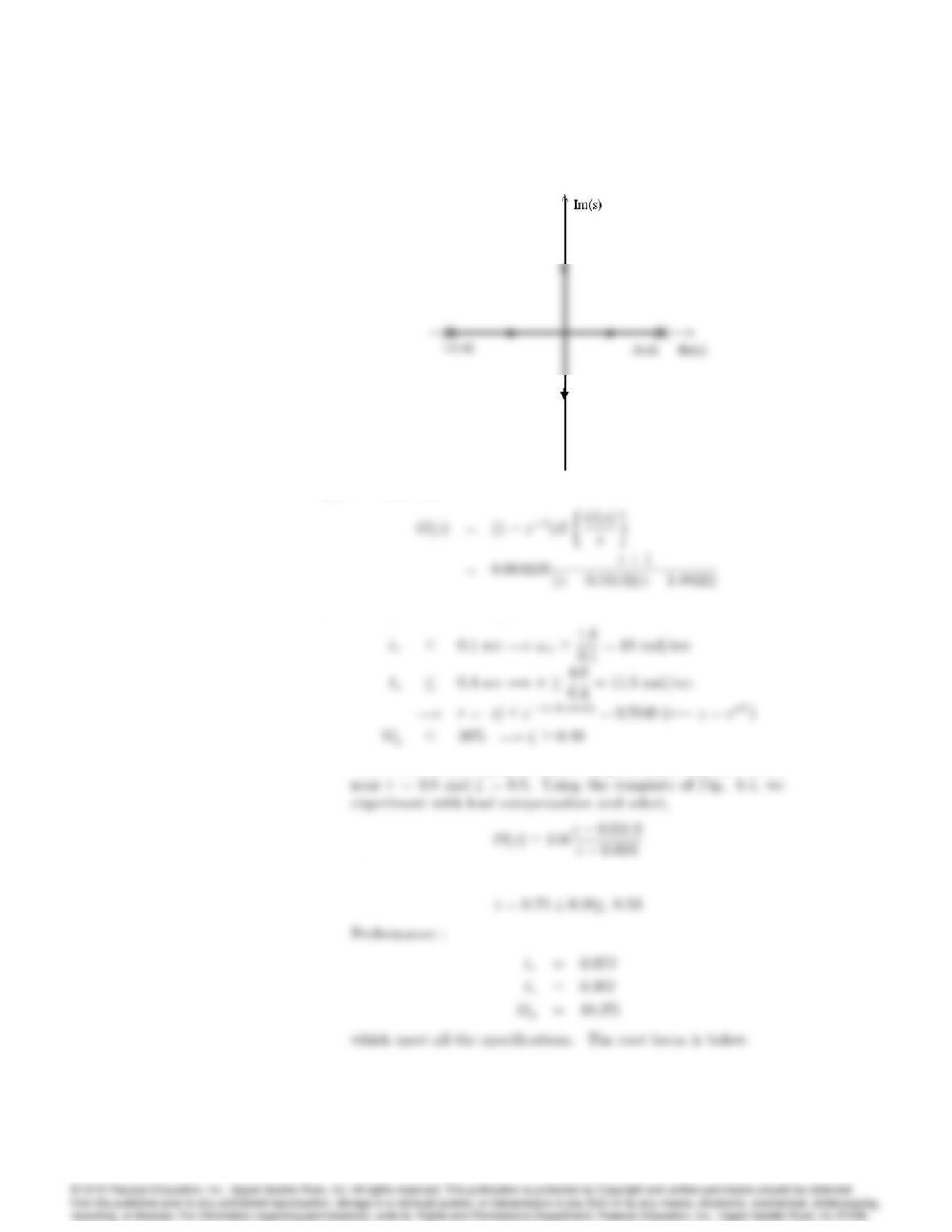
(a) Compute the transfer function from Ito x, and draw the (continuous)

root locus for the simple feedback i=Kx.

(b) Assume the input is passed through a ZOH, and let the sampling

period be 0.02 sec. Compute the transfer function of the equivalent

discrete-time plant.

(c) Design a digital control for the magnetic levitation device so that the

closed-loop system meets the following specifications: tr0:1 sec,

ts0:4 sec, and overshoot 20%.

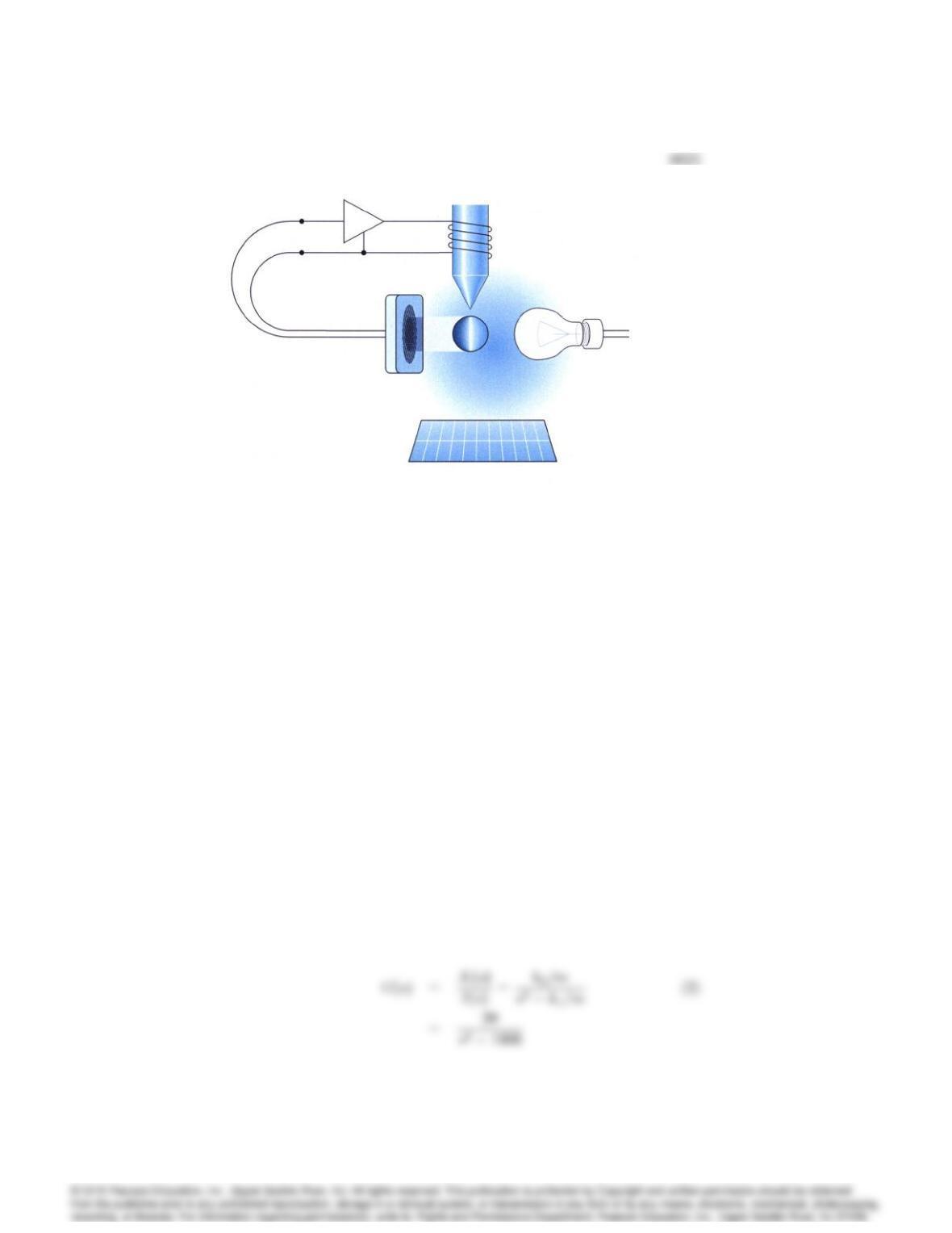
Figure 8.25: Schematic of magnetic levitation device for Problem 8.11

(d) Plot a root locus with respect to k1for your design, and discuss the

possibility of using your closed-loop system to balance balls of various

masses.

(e) Plot the step response of your design to an initial disturbance dis-

placement on the ball, and show both xand the control current i.

If the sensor can measure xonly over a range of 1=4cm and the

amplifier can only provide a current of 1 A, what is the maximum

displacement possible for control, neglecting the nonlinear terms in

f(x; I)?

Solution:

(a)

8026 CHAPTER 8. DIGITAL CONTROL

(b) T= 0:02 sec,

(c) The specifications imply that :

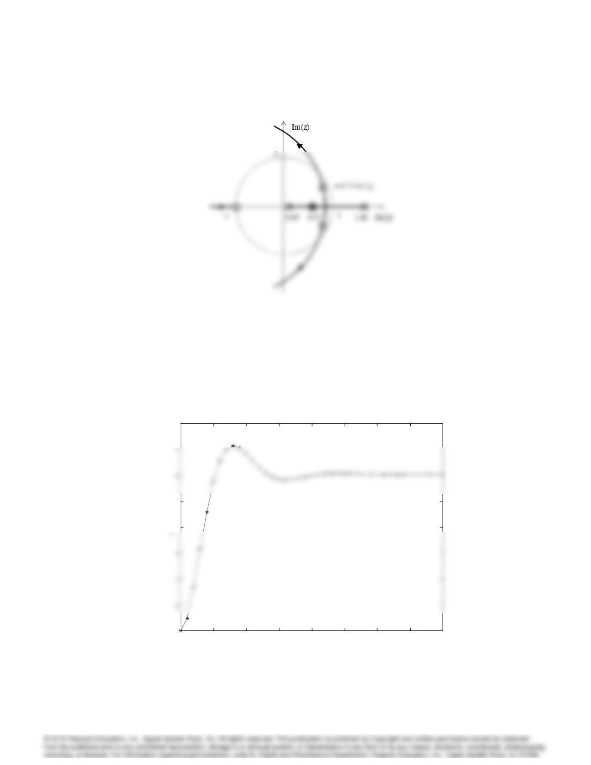
Thus, the closed-loop poles must be pulled into the unit circle

The closed-loop poles are :

8027

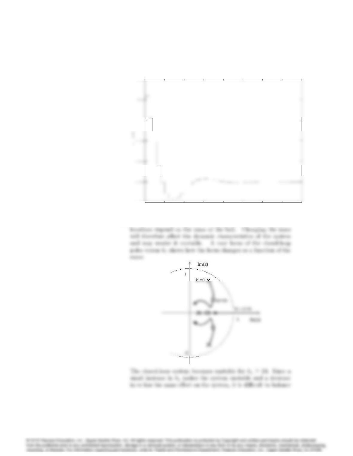
The step response shows Mp

00.1 0.2 0.3 0.4 0.5 0.6 0.7 0.8

0

4

5

8

Closed-Loop Step Response

Time (sec)

8028 CHAPTER 8. DIGITAL CONTROL

00.1 0.2 0.3 0.4 0.5 0.6 0.7 0.8

-400

0

200

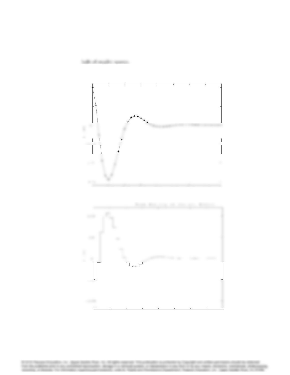
Time History of Control Effort

Time (sec)

(d) As can be seen from Eq. (2), the loop gain and the open loop pole

8029

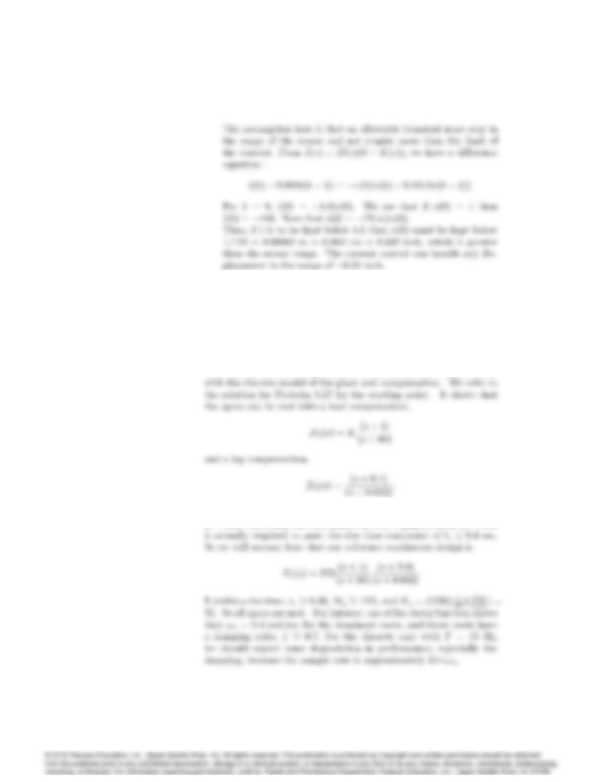
(e) The response to an initial xdisplacement is shown :

00.1 0.2 0.3 0.4 0.5 0.6 0.7 0.8

0.5

1

Closed-Loop Initial Response

Time (sec)

00.1 0.2 0.3 0.4 0.5 0.6 0.7 0.8

Time (sec)

8030 CHAPTER 8. DIGITAL CONTROL

12. Repeat Problem 5.27 in Chapter 5 by constructing discrete root loci

and performing the designs directly in the z-plane. Assume that the

output yis sampled, the input uis passed through a ZOH as it enters

the plant, and the sample rate is 15 Hz.

Solution

(a) The most effective discrete design method is to start with some idea

what the continuous design looks like, then adjust that as necessary

Although it is stated in the solution to Problem 5.27 that a gain,

K= 240 will satisfy the constraints, in fact, a gain of about K= 270

8031

The discrete transfer function for the plant described by G(s)and

preceded by a ZOH is:

which produces:

which for T= 1=15 = 0:0667 and TD= 1 reduces to

8032 CHAPTER 8. DIGITAL CONTROL

The time response of the final design below shows that all specs are

met.

0.2

0.6

1.2

y

Step Response

13. Design a digital controller for the antenna servo system shown in Figs. 3.60

and 3.61 and described in Problem 3.36. The design should provide a step

response with an overshoot of less than 10% and a rise time of less than

80 sec.

(a) What should the sample rate be?

(b) Use the matched pole-zero discrete equivalent method.

(c) Use discrete design and the z-plane root locus.

Solution

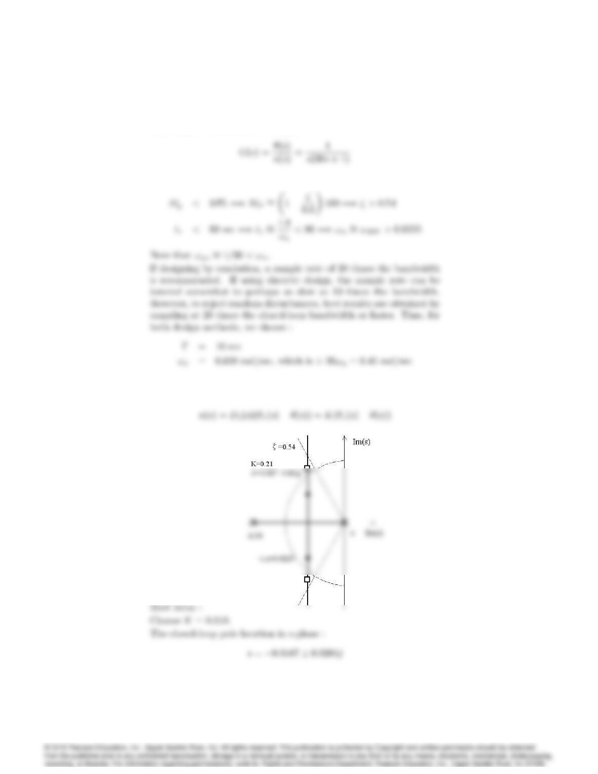
(a) The equation of motion is :

8033

after Laplace transform, we obtain :

From the specifications,

(b) Continuous design :

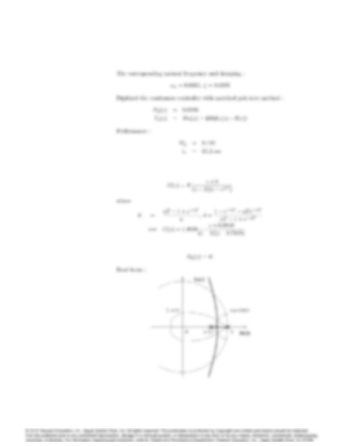
Use a proportional controller :

8034 CHAPTER 8. DIGITAL CONTROL

(c) With u(k)applied through a ZOH, the transfer function for an equiv-

alent discrete-time system is :

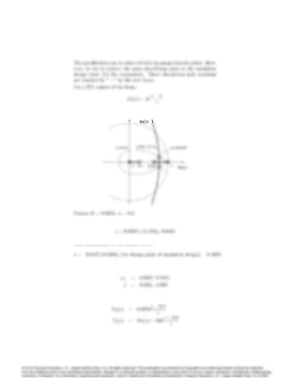
Use a proportional control of the form :

8035

Root locus :

The resulting z-plane roots :

which satisfy the specification :

The control law :

8036 CHAPTER 8. DIGITAL CONTROL

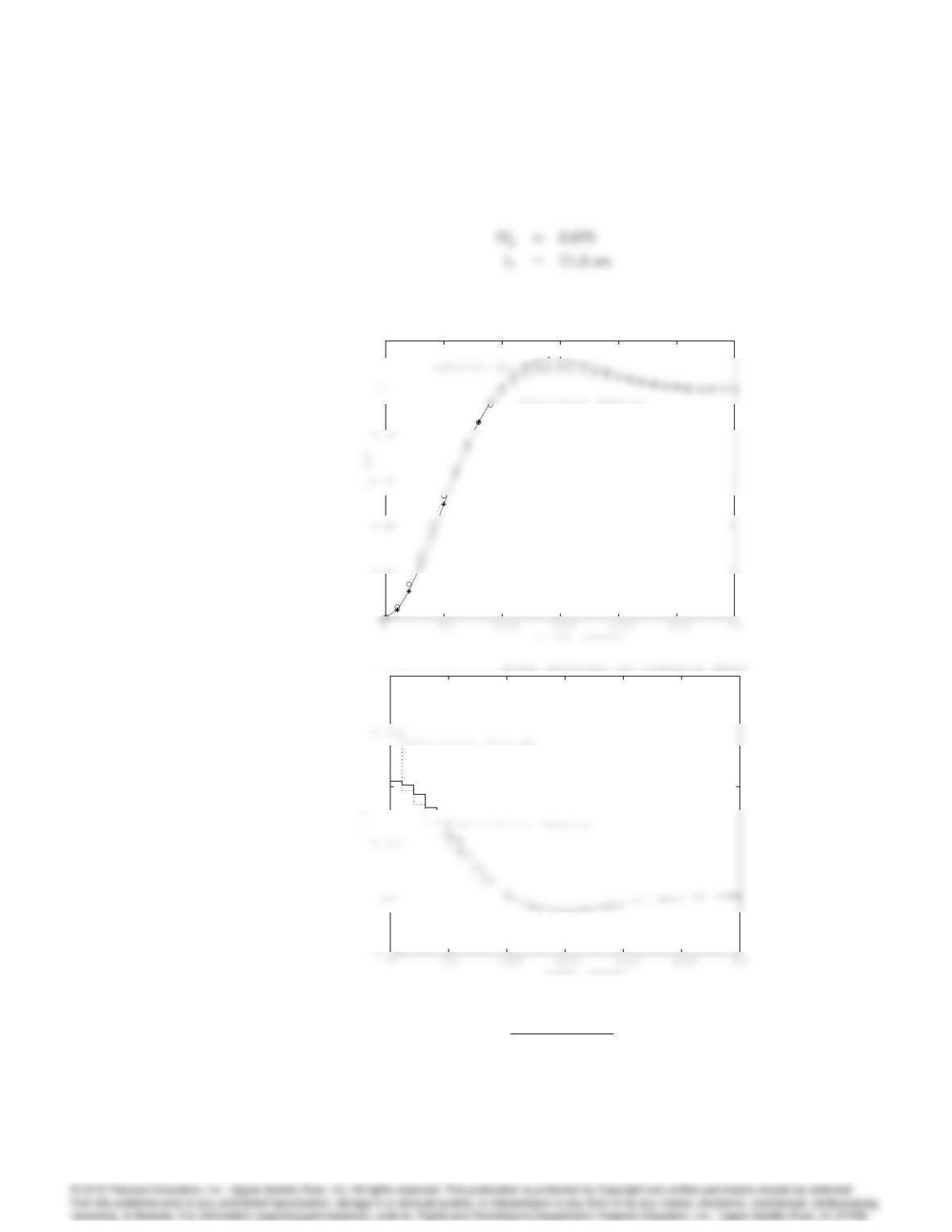
Performance :

Step response :

0.2

1.2

Step Response

0.02

0.04

14. The system

G(s) = 1

(s+ 0:1)(s+ 3)

8037

is to be controlled with a digital controller having a sampling period of

T= 0:1sec. Using a z-plane root locus, design compensation that will

respond to a step with a rise time tr1sec and an overshoot Mp5%.

What can be done to reduce the steady-state error?

Solution

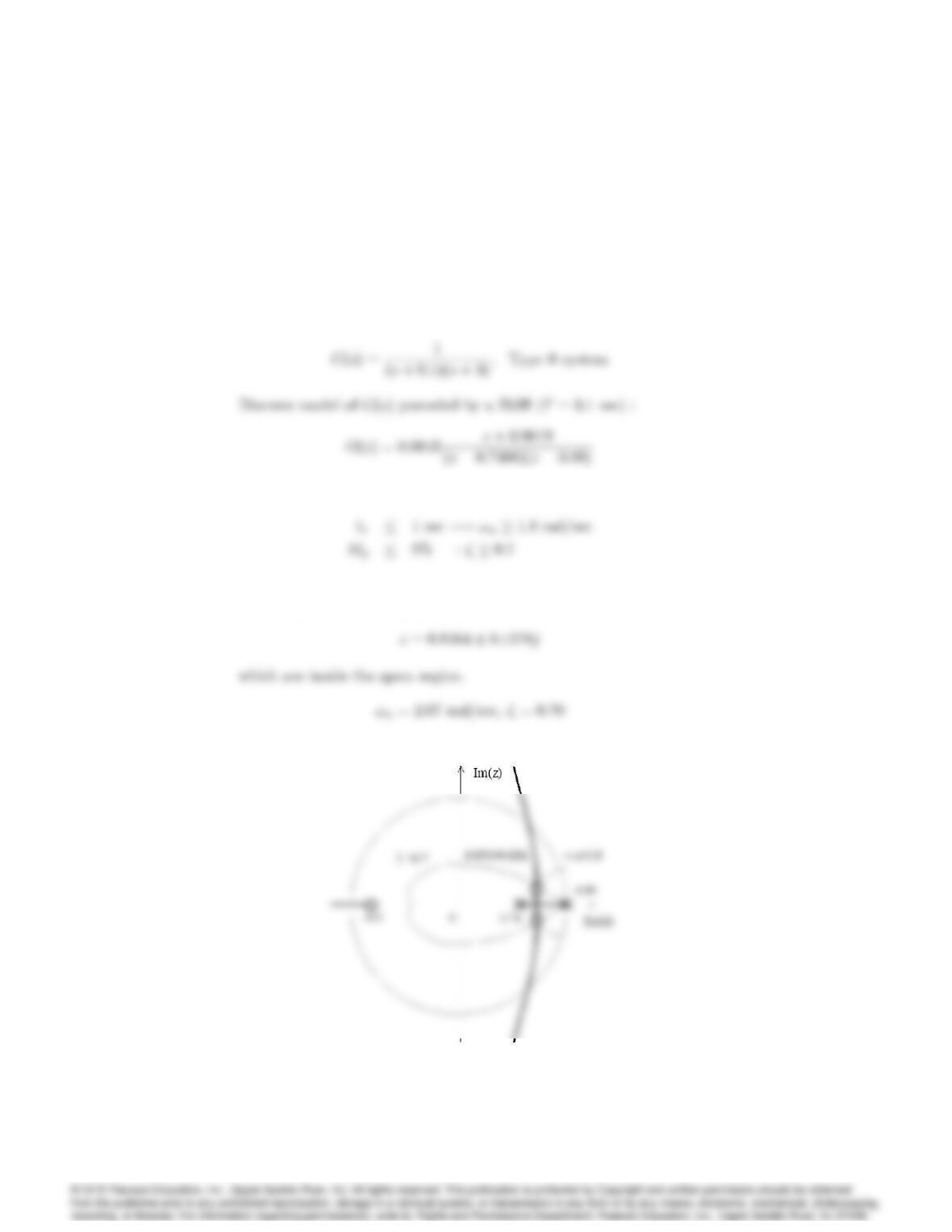
(a) Continuous plant :

Specifications :

Discrete design : A simple proportional feedback, D(z) = K= 4:0,

will bring the closed-loop poles to :

Root locus :

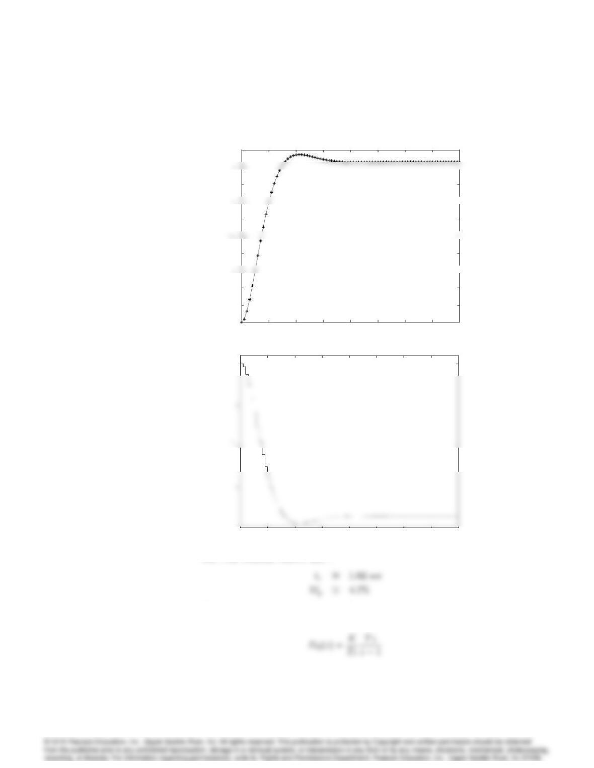
8038 CHAPTER 8. DIGITAL CONTROL

Step response :

0 1 2 3 4 5 6 7 8

0

0.1

0.2

0.4

0.6

0.8

1

Closed-Loop Step Response

Time (sec)

0 1 2 3 4 5 6 7 8

0

2

4

Time History of Control Effort

Time (sec)

The step response shows that :

However, since the system is type 0, steady-state error exists and is

7% in this case. An integral control of the form,

15. The transfer function for pure derivative control is

Dd(z) = KTD

z1

T z ;

where the pole at z= 0 adds some destabilizing phase lag. Can this phase

lag be removed by using derivative control of the form

Dd(z) = KTD

(z1)

T?

Support your answer with the difference equation that would be required,

and discuss the requirements to implement it.

Solution:

(a) No, we cannot use derivative control of the form :