Operating Systems Chapter 7 Homework Write the dynamic equations describing the circuit in Fig

Solutions Manual: Chapter 7

7th Edition

Feedback Control of Dynamic

Systems

Gene F. Franklin

J. David Powell

Abbas Emami-Naeini .

Assisted by:

H.K. Aghajan

H. Al-Rahmani

P. Coulot

P. Dankoski

S. Everett

R. Fuller

T. Iwata

V. Jones

F. Safai

L. Kobayashi

H-T. Lee

E. Thuriyasena

M. Matsuoka

J.K. Lee

1

h t 7

t t i n

Problems and Solutions for Section . : lock diagrams and

State S ace

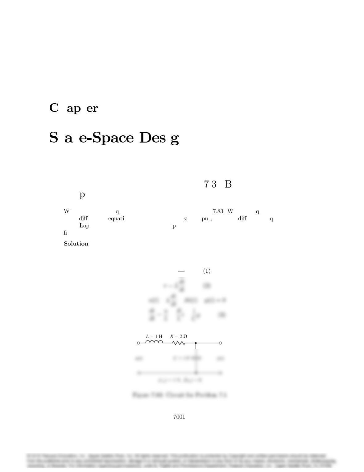
1. rite the dynamic e uations describing the circuit in Fig. rite the e uations as a second-

order erential on in y(t). Assuming a ero in t solve the erential e uation for y(t)

using lace-transform methods for the arameter values and initial conditions shown in the

gure. Verify your answer using the initial command in Matlab.

:

i=Cdy

7002 CHAPTER 7. STATE-SPACE DESIGN

Substituting the given values for L,R, and Cwe have for equation (3):

Characteristic equation:

Solving for the coe¢cients:

y(t) = A1et+A2tet

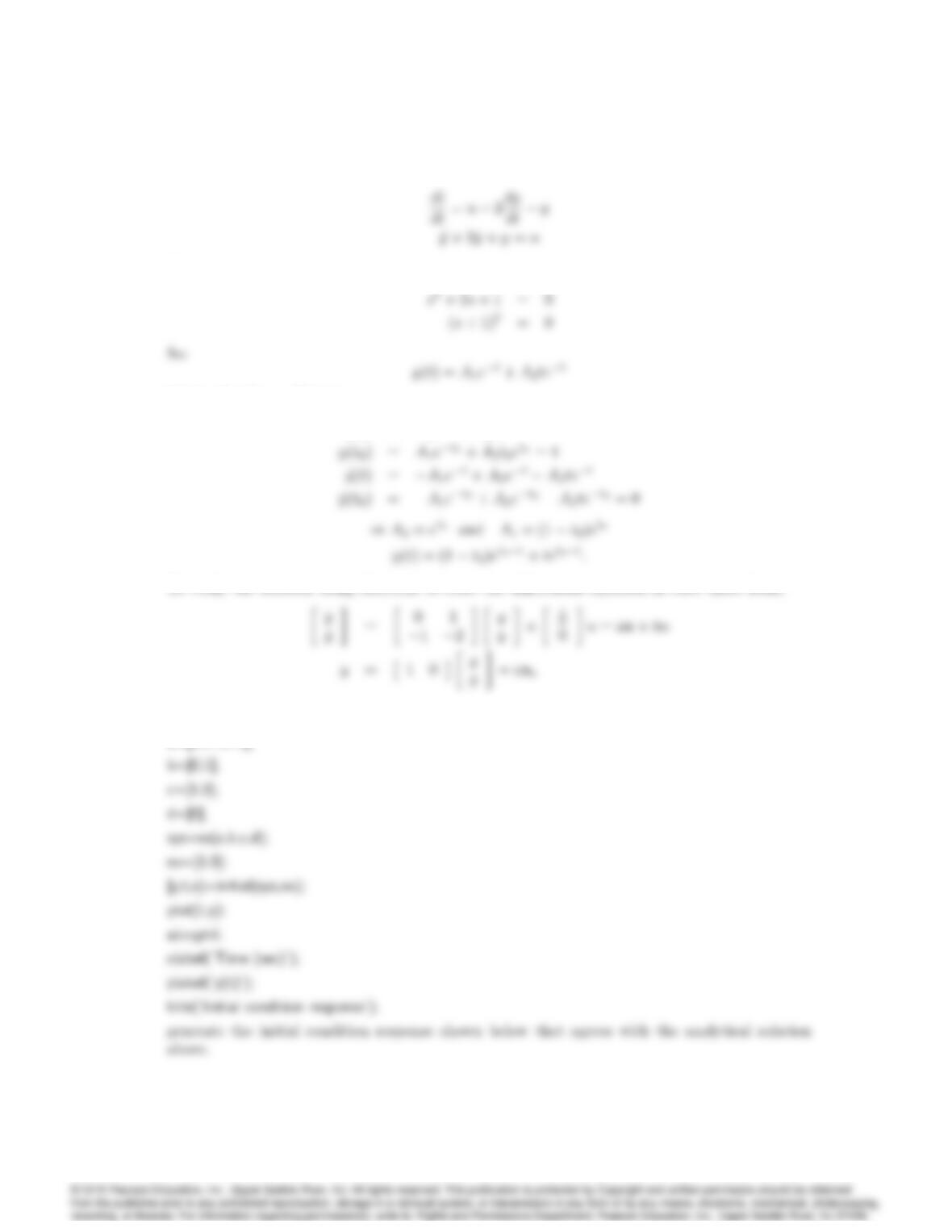
To verify the solution using Matlab, re-write the di¤erential equation in state space form,

where x= [y:

y]T.L= 1. Then the following Matlab statements,

a=[0,1;-1,-2];

7003

0 2 4 6 8 10

0.4

0.6

0.8

1

Time (sec)

Initial condition response

0 2 4 6 8 10

0.4

0.6

0.8

1

Time (sec)

Initial condition response

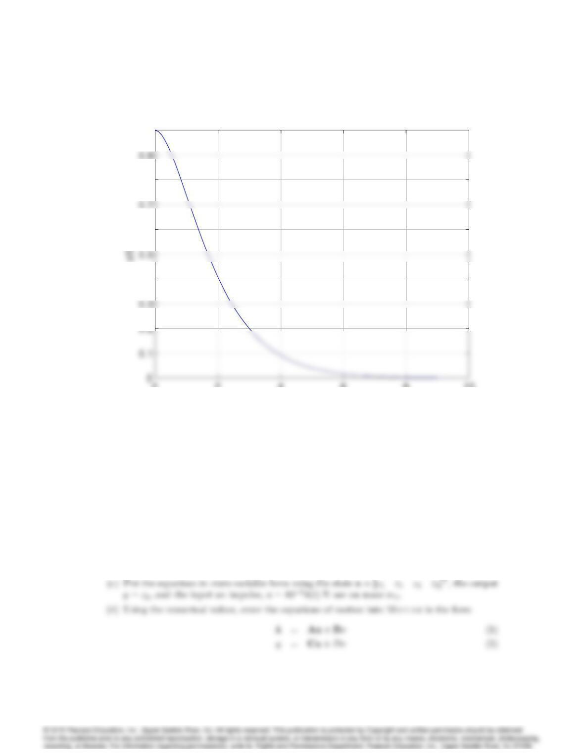
Problem 7.1: Initial condition response.

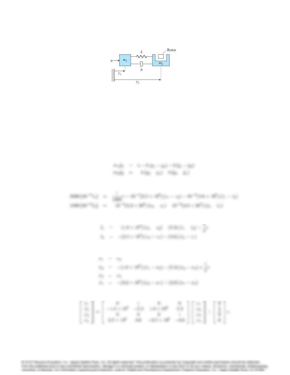
2. A schematic for the satellite and scientific probe for the Gravity Probe-B (GP-B) experiment

that was launched on April 30, 2004 is sketched in Fig. 7.84. Assume that the mass of the

spacecraft plus helium tank, m1, is 2000 kg and the mass of the probe, m2, is 1000 kg. A

rotor will ‡oat inside the probe and will be forced to follow the probe with a capacitive forcing

mechanism. The spring constant of the coupling, k, is 3:2106. The viscous damping bis

4:6103:

(a) Write the equations of motion for the system consisting of masses m1and m2using the

inertial position variables, y1and y2.

(b) The actual disturbance uis a micrometeorite, and the resulting motion is very small

Therefore, rewrite your equations with the scaled variables z1= 106y1,z2= 106y2, and

v= 1000u:

7004 CHAPTER 7. STATE-SPACE DESIGN

Figure 7.84: Schematic diagram of the GP-B satellite and probe.

and define the Matlab system: sysGPB = ss(A,B,C,D). Plot the response of ycaused by

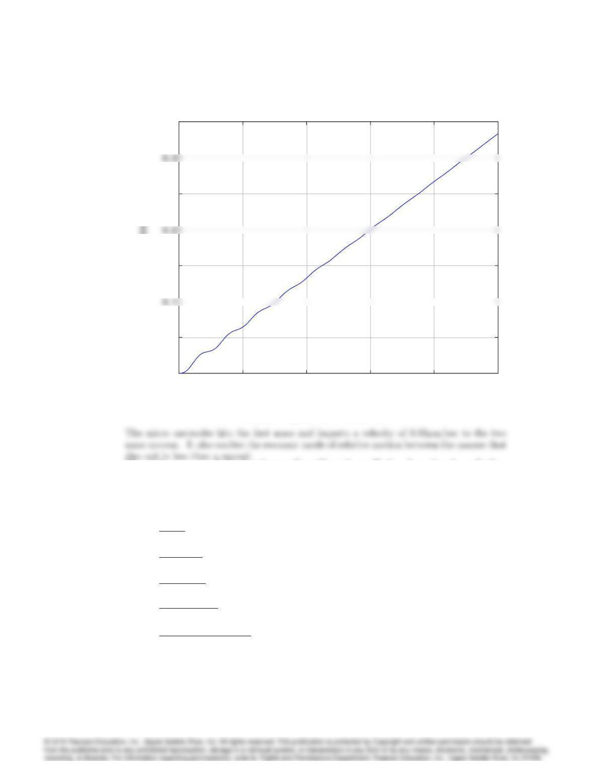
the impulse with the Matlab command impulse(sysGPB). This is the signal the rotor must

follow.

(e) Use the Matlab commands p = eig(A) to find the poles (or roots) of the system and z =

tzero(A,B,C, D) to find the zeros of the system.

Solution:

(a) The rotor is not part of the problem and can be ignored in writing the equations of

motion

(b) Let’s put in the values for the parameters as well as scale the variables as requested.

which becomes

(c) The state-variable form for x= [z1_z1z2_z2]Tis

or, in matrix form

7005

and the output equation is

(d) The system matrices

plus the Matlab statements:

7006 CHAPTER 7. STATE-SPACE DESIGN

00.2 0.4 0.6 0.8 1

0

0.05

0.15

0.25

0.35

Time (sec)

y2 (micro-meters)

impulse response of y

2

00.2 0.4 0.6 0.8 1

0

0.05

0.15

0.25

0.35

Time (sec)

y2 (micro-meters)

impulse response of y

2

Impulse response for Problem 7.2.

Problems and Solutions for Section 7.4: Analysis of the

State Equations

3. Give the state description matrices in control-canonical form for the following transfer functions:

(a) G(s) = 1

2s+ 1:

(b) G(s) = 6(s=3 + 1)

(s=10 + 1):

(c) G(s) = 8s+ 1

s2+ 3s+ 2:

(d) G(s) = s+ 7

s(s2+ 2s+ 2):

(e) G(s) = (s+ 10)(s2+s+ 25)

s2(s+ 2)(s2+s+ 36):

Solution:

7007

(d)

(e)

2

3

2

3

4. Use the Matlab function tf2ss to obtain the state matrices called for Problem 7.3.

Solution:

In all cases, simply form num and den given below and then use the Matlab command [A,B,C,D]

= tf2ss(num,den).

5. Give the state description matrices in normal-mode form for the transfer functions of Prob-

lem 7.3. Make sure that all entries in the state matrices are real valued by keeping any pairs

of complex conjugate poles together, and realize them as a separate subblock in control canoni-

cal form.

Solution:

(b) A=10; B = 1; C =140; D = 20:

(c) 8s+ 1

7008 CHAPTER 7. STATE-SPACE DESIGN

(d)

The computation can also be done using the residue command in Matlab:[r,p,k]=residue(num,den).

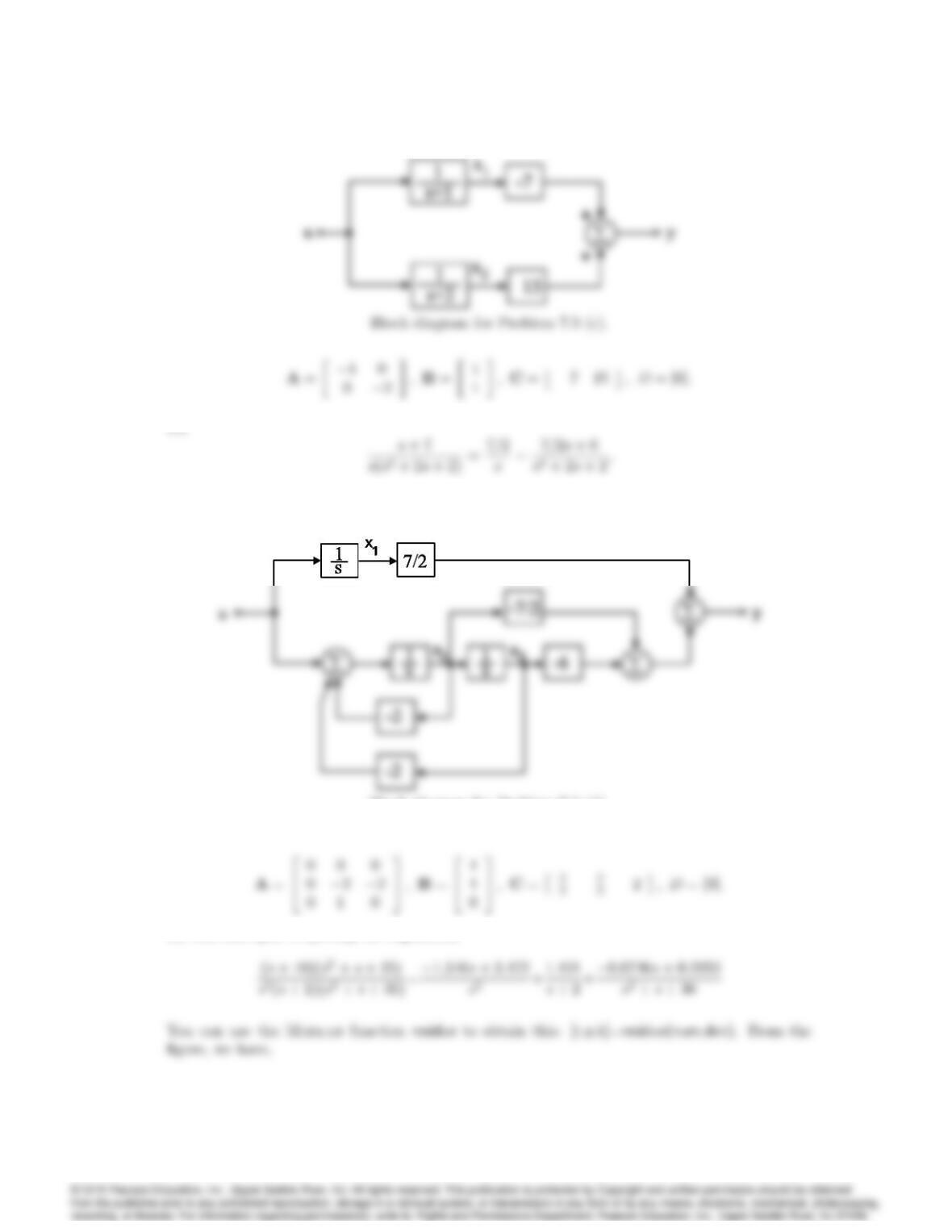
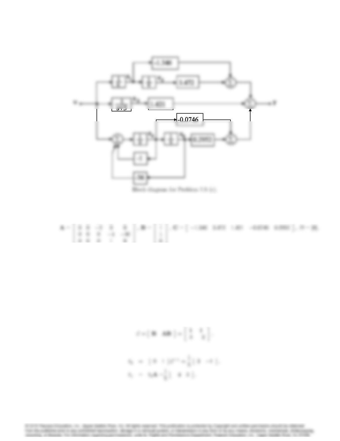
Block diagram for Problem 7.5 (d).

(e) The hard part is getting the expansion,

7009

2

6

0 0 0 0 0

1 0 0 0 0

3

7

2

6

1

0

3

7

6. A certain system with state xis described by the state matrices,

A=2 1

2 0 ;B=1

3;

C= [ 1 0 ]; D = 0:

Find the transformation Tso that if x=Tz, the state matrices describing the dynamics of z

are in control canonical form. Compute the new matrices 

A,

B,C, and 

D.

Solution:

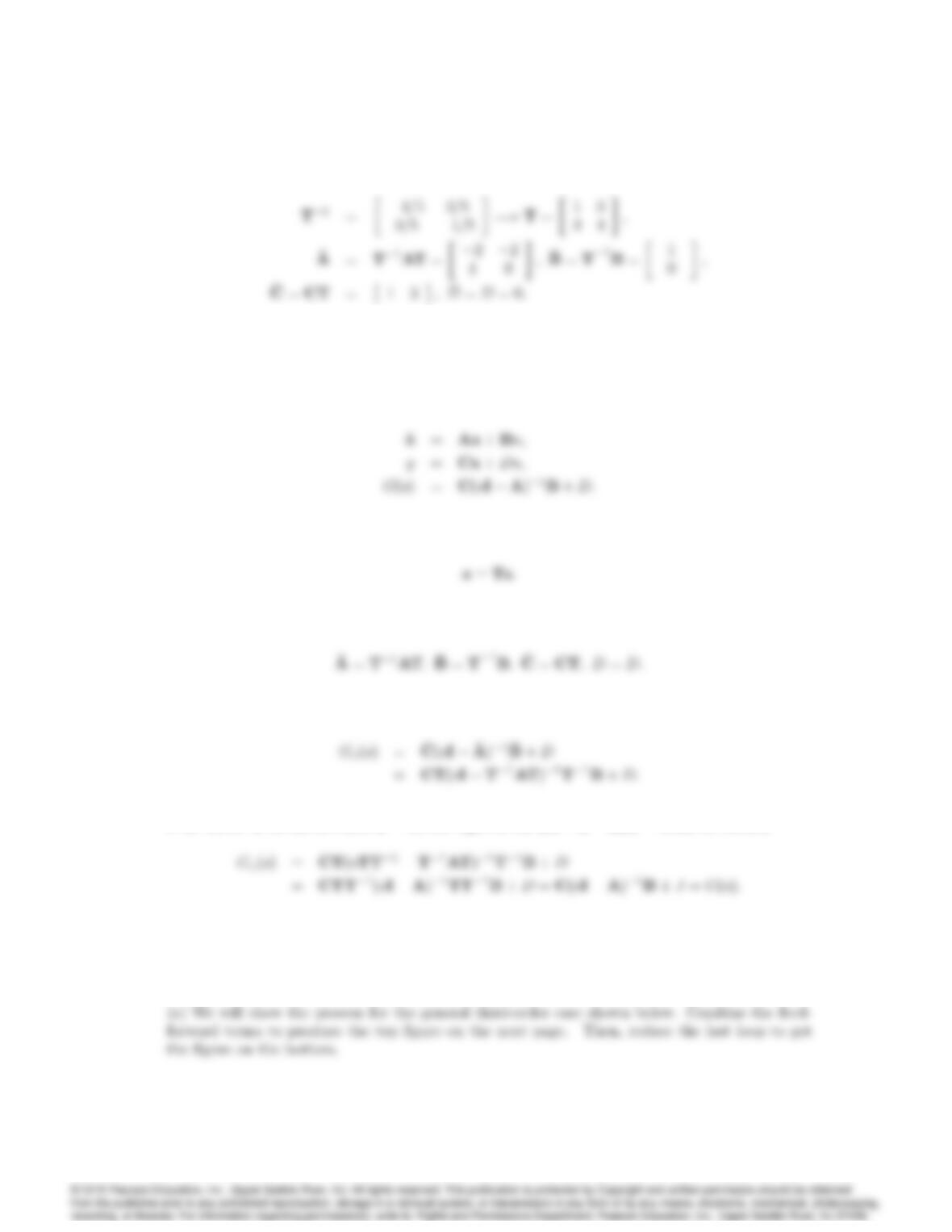
Following the procedure outlined in the chapter, we have,

7010 CHAPTER 7. STATE-SPACE DESIGN

Thus,

7. Show that the transfer function is not changed by a linear transformation of state.

Solution:

Assume the original system is,

Assume a change of state from xto zusing the nonsingular transformation T;

The new system matrices are,

The transfer function is,

If we factor Ton the left and T1on the right of the (sIT1AT)1term, we obtain,

8. Use block-diagram reduction or Mason’s rule to find the transfer function for the system in

observer canonical form depicted by Fig. 7.31.

Solution:

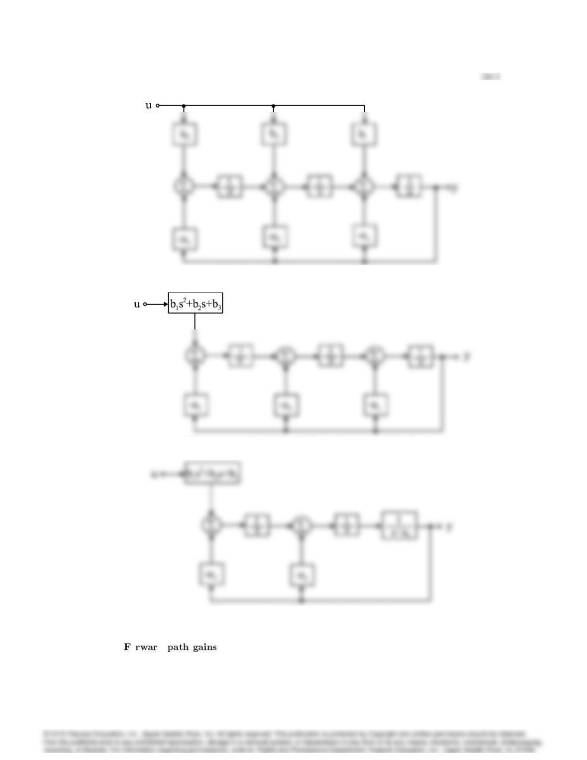
Problem 7.8: Observer canonical form.

Observer canonical form: feedforward terms combined.

Observer canonical form: one loop reduced.

(a) Using Mason’s rule:

o d :

7012 CHAPTER 7. STATE-SPACE DESIGN

9. Suppose we are given a system with state matrices A;B;C(D= 0 in this case). Find the

transformation Tso that, under Eqs. (7.21) and (7.22), the new state description matrices will

be in observer canonical form.

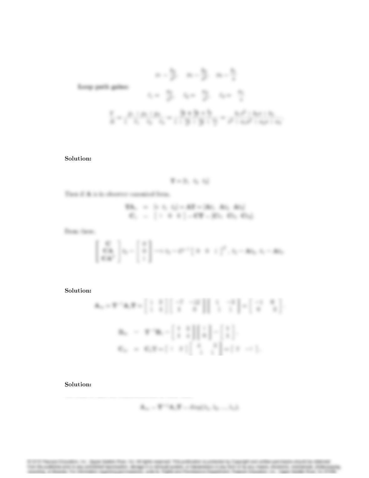
Express the transformation matrix in terms of its column vectors,

10. Use the transformation matrix in Eq. (7.38) to explicitly multiply out the equations at the end

of Example 7.9.

11. Find the state transformation that takes the observer canonical form of Eq. (7.32) to the modal

canonical form.

We wish to find the transformation Tsuch that,

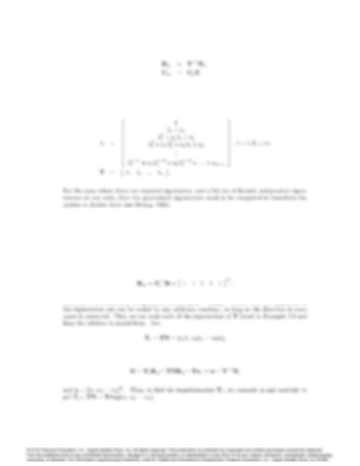
7013

The columns of Tare the eigenvectors of Ao. The eigenvectors of Aoare all of the form (which

can be proved by induction):

12. a) Find the transformation Tthat will keep the description of the tape-drive system of Ex-

ample 7.10 in modal canonical form but will convert each element of the input matrix Bmto

unity.

b) Use Matlab to verify that your transformation does the job.

Solution:

(a) We would like to find a transformation matrix T1such that,

Since T1is full rank, this is equivalent to solving B=T1Bm. Recall that the magnitude of

where tiare the eigenvectors, niare scalars and N=diag(n1,   ,n5). Now,

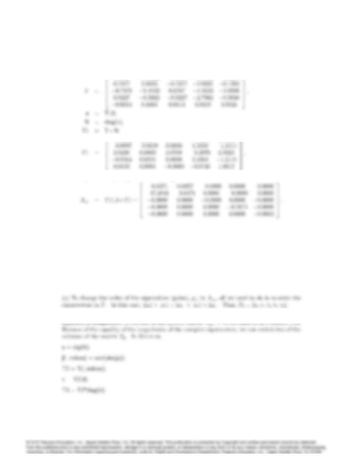
7014 CHAPTER 7. STATE-SPACE DESIGN

(b) In Matlab,

2

1:4708 0:17221 1:4708 1:5432 3:3237

3

2

0:3883 0:0247 2:8708 4:8234 2:3162

3

Bm=T1nB=11111T;

13. a) Find the state transformation that will keep the description of the tape-drive system of

Example 7.10 in modal canonical form but will cause the poles to be displayed in Amin order

of increasing magnitude.

b) Use Matlab to verify your result in part (a), and give the complete new set of state matrices

as A,B,C, and D.

Solution:

(b) Our solution uses the Matlab sort command to re-order eigenvectors. Note that this

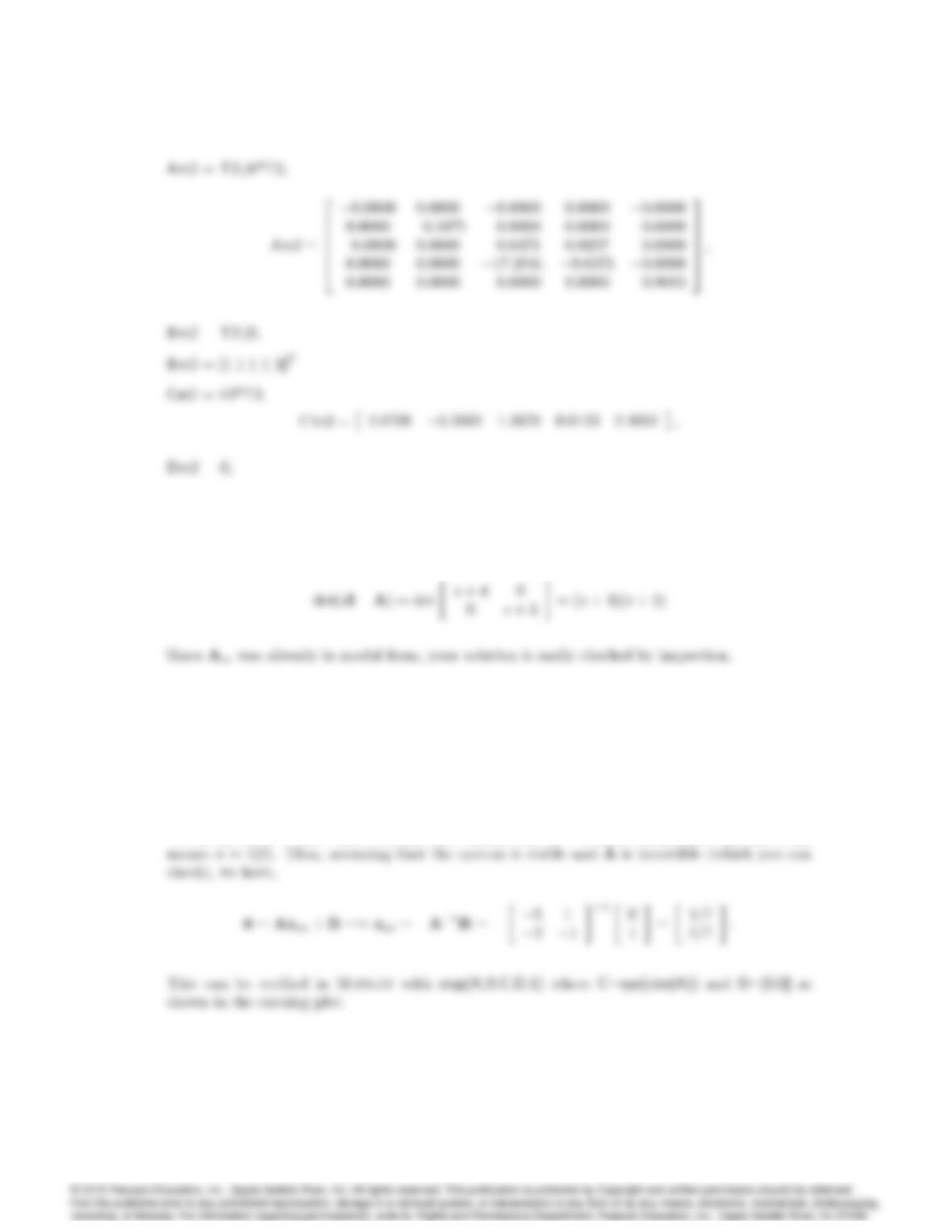
7015

14. Find the characteristic equation for the modal-form matrix Amof Eq. (7.14a) using Eq. (7.55).

Solution:

15. Given the system,

_

x=5 1

21x+0

1u;

with zero initial conditions, find the steady-state value of xfor a step input u.

Solution:

We are given _x =Ax +Bu. Steady-state means that _x = 0 and a step input (or unit step)

7016 CHAPTER 7. STATE-SPACE DESIGN

0

0.05

0.2

00.5 11.5 22.5 33.5 44.5

0

Step Response

0

0.05

0.2

00.5 11.5 22.5 33.5 44.5

0

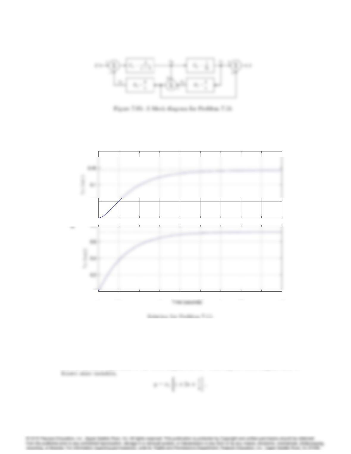
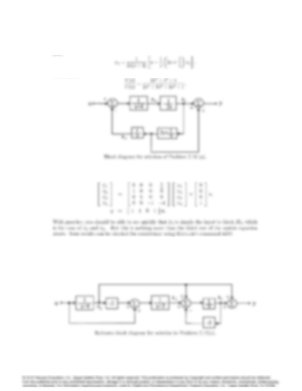
16. Consider the system shown in Fig. 7.85:

a) Find the transfer function from Uto Y.

b) Write state equations for the system using the state variables indicated.

Solution:

(a) The system is equivalent to the block diagram shown. Following the block diagram back to

7017

resulting in,

Another possible solution is in terms of Mason’s rule.

(b)

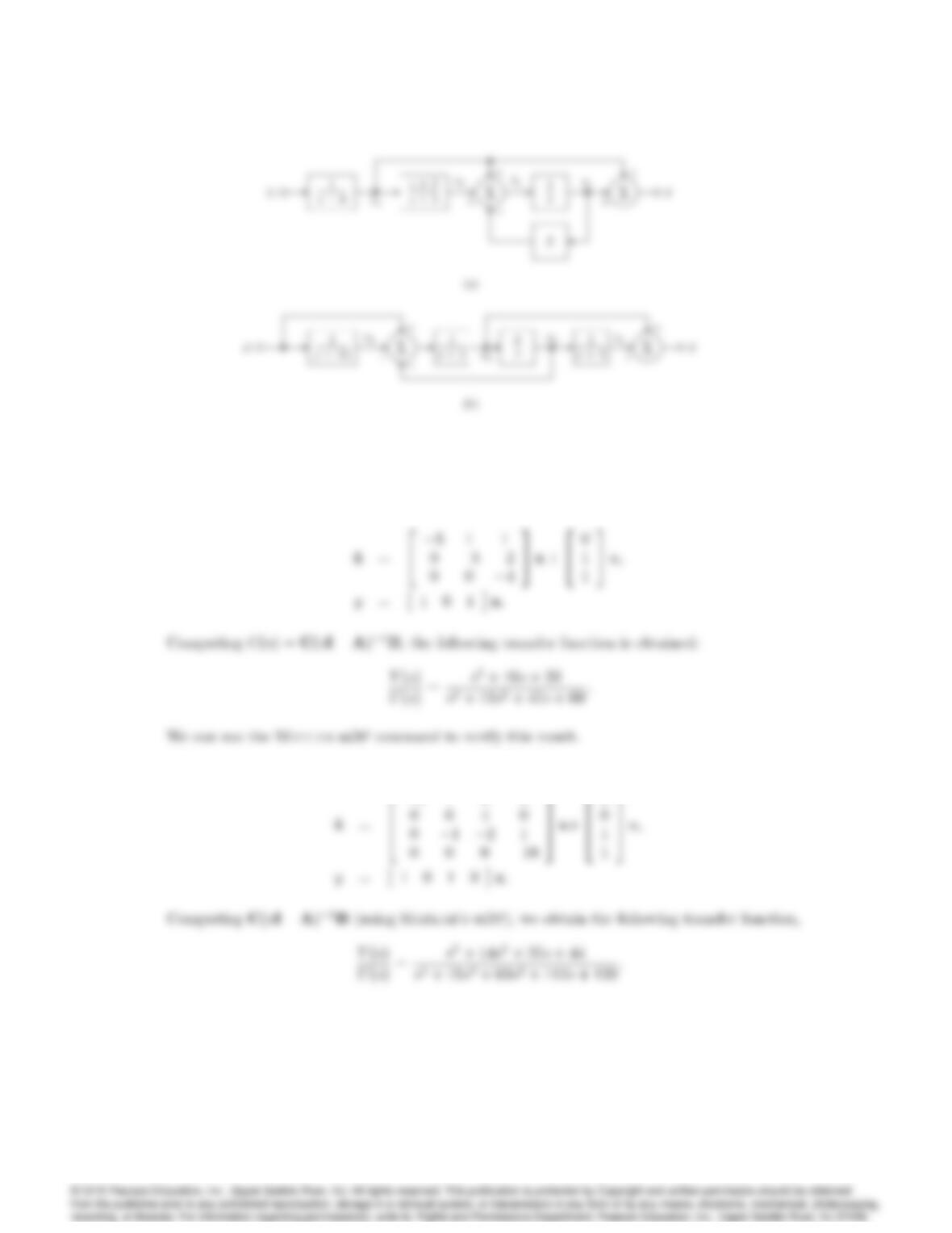
17. Using the indicated state variables, write the state equations for each of the systems shown in

Fig. 7.86. Find the transfer function for each system using both block-diagram manipulation

and matrix algebra [as in Eq. (7.45)].

Solution:

(a) Performing a partial fraction expansion on (s+ 2)=(s+ 4), Fig. 7.86(a) can be redrawn as

shown below.

7018 CHAPTER 7. STATE-SPACE DESIGN

Figure 7.86: Block diagrams for Problem 7.17.

By inspection of the block diagram, the state equations are,

(b) Using the second block diagram given in Fig. 7.86(b), we can write,

3 1 0 0

3

0

3

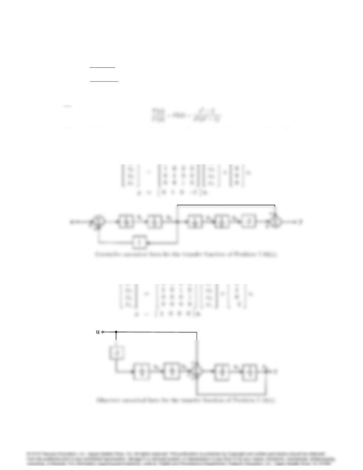
18. For each of the listed transfer functions, write the state equations in both control and observer

canonical form. In each case draw a block diagram and give the appropriate expressions for A,

B, and C.

7019

a)G(s) = s22

s2(s21) (control of an inverted pendulum by a force on the cart)

b)G(s) = 3s+ 4

s2+ 2s+ 2

Solution:

This transfer function can be realized in controller canonical form as shown below. From the

figure, we have,

2

_x1

3

0100

3

x1

3

1

3

The block diagram for observer canonical form is shown below. From the figure, we have,

2

3