7040 CHAPTER 7. STATE-SPACE DESIGN
Since the system is Type I, its DC gain is unity, so that
33. Prove that the Nyquist plot for LQR design avoids a circle of radius one centered at the -1 point
as shown in Fig. 7.89. Show that this implies that 1
2<GM<1the “upward” gain margin is
GM =1;and there is a “downward” GM=1
2, and the phase margin is at least PM =60.
Hence the LQR gain matrix, K, can be multiplied by a large scalar or reduced by half with
guaranteed closed-loop system stability.
Solution:
It has been proved (Anderson and Moore, 1990) that the Nyquist plot for LQR design avoids a
circle of radius one centered at the 1point as shown in Fig. 7.89. This leads to extraordinary
7041
phase and gain margin properties as shown below. First note that the state-feedback system
can be re-drawn in the usual feedback configuration as shown on the next page. Using Eq.
(7.72) and factoring (sIA), we have
Now1, using the above equation and Eq. (7.95) we can write,
Setting s=j! we obtain,
Finally, Eq. (8) implies that,
which means that the Nyquist plot must indeed avoid a circle centered at 1with unit radius.
The Nyquist plot approaches the origin for large frequencies, and we find that the “upward”
7042 CHAPTER 7. STATE-SPACE DESIGN
Problems and Solutions for Section 7.7: Estimator Design
34. Consider the system
A=2 1
1 0 ;B=1
0;C= [1 2];
and assume that you are using feedback of the form u=Kx +r, where ris a reference input
signal.
a) Show that (A,C) is observable.
b) Show that there exists a Ksuch that (ABK,C)is unobservable.
c) Compute a Kof the form K= [1; K2]that will make the system unobservable as in part (b);
that is, find K2so that the closed-loop system is not observable.
d) Compare the open-loop transfer function with the transfer function of the closed-loop system
of part (c). What is the unobservability due to?
Solution:
(a)
(b) Let,
(d)
7043
35. Consider a system with the transfer function,
G(s) = 9
s29:
a) Find (Ao,Bo,Co) for this system in observer canonical form.
b) Is (Ao,Bo) controllable?
c) Compute Kso that the closed-loop poles are assigned to s=33j.
d) Is the closed-loop system of part (c) observable?
e) Design a full-order estimator with estimator-error poles at s=12 12j.
f) Suppose the system is modified to have a zero:
G1(s) = 9(s+ 1)
s29:
Prove that if u=Kx +r, there is a feedback gain Kthat makes the closed-loop system
unobservable. [Again assume an observer canonical realization for G1(s).]
Solution:
(a) For a transfer function,
(b) To check whether (Ao;Bo)is controllable we form the controllability matrix,
(d) The system is in observer canonical form. Hence, it is guaranteed to be observable. To
check,
7044 CHAPTER 7. STATE-SPACE DESIGN
in observer canonical form yields,
by a zero.
36. Explain how the controllability, observability, and stability properties of a linear system are
related.
Solution:
controllability =)det [B AB A2BAn1B]6= 0:
37. Consider the electric circuit shown in Fig. 7.90.
a) Write the internal (state) equations for the circuit. The input u(t)is a current, and the
output yis a voltage. Let x1=iLand x2=vc.
b) What condition(s) on R,L, and Cwill guarantee that the system is controllable?
c) What condition(s) on R,L, and Cwill guarantee that the system is observable?
Solution:
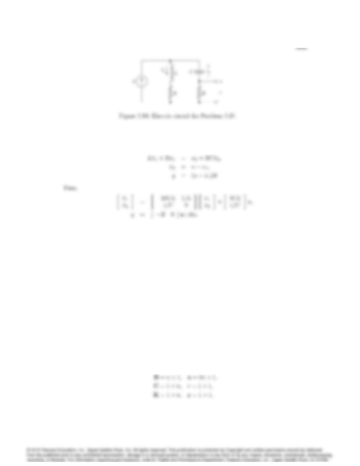
(a) Apply Kirchhoff’s voltage and current laws, with x1=iLand x2=vc, we obtain,
(b) The condition for the system to be uncontrollable is det(C) =0.
C=B AB =R=L 2R2=L2+ 1=LC
1=C R=LC :
det(C) = R2=L2C1=LC2:
Thus, the system is controllable if R26=L=C.
(c) The condition for the system to be unobservable is,
O=C
CA =R0
2R2=L R=L :
det(O) = R2=L:
Since det(O)6= 0 for any R; L; C except R= 0 or L=1, the system is observable.
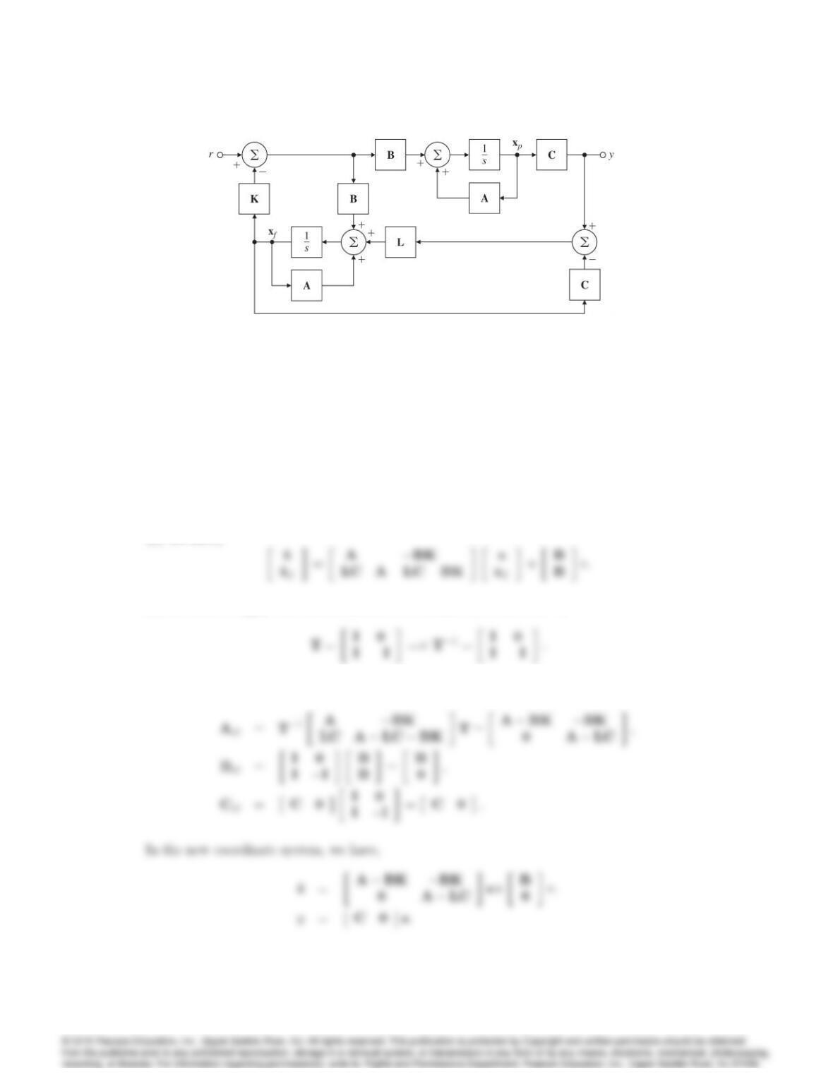
38. The block diagram of a feedback system is shown in Fig. 7.91. The system state is,
x=xp
xf;
and the dimensions of the matrices are as follows:
A=nn; L=n1;
7046 CHAPTER 7. STATE-SPACE DESIGN
Figure 7.91: Block diagram for Problem 7.38.
a) Write state equations for the system.
b) Let x=Tz, where
T=I 0
II:
Show that the system is not controllable.
c) Find the transfer function of the system from rto y.
Solution:
(a) We have, _x
(b) In order to apply our transformation of coordinates, we need T1,
Thus,
we have shown that it is an uncontrollable system.
(c) The transfer function is,
39. This problem is intended to give you more insight into controllability and observability. Consider
the circuit in Fig. 7.92, with an input voltage source u(t)and an output current y(t).
a) Using the capacitor voltage and inductor current as state variables, write state and output
equations for the system.
b) Find the conditions relating R1,R2,C, and Lthat render the system uncontrollable. Find
a similar set of conditions that result in an unobservable system.
c) Interpret the conditions found in part (b) physically in terms of the time constants of the
system.
d) Find the transfer function of the system. Show that there is a pole-zero cancellation for the
conditions derived in part (b) (that is, when the system is uncontrollable or unobservable).
Solution:
(a) From Figure 7.92,
(b) First, form the controllability matrix,
7048 CHAPTER 7. STATE-SPACE DESIGN
(c) When the system is unobservable/uncontrollable, we have 1=R1C=R2=L so that:
(d)
Ls+1
LC
40. The linearized equations of motion for a satellite are,
_x =Ax +Bu;
y=Cx;
where
A=2
6
6
4
0 1 0 0
3!20 0 2!
0 0 0 1
02!0 0
3
7
7
5;B=2
6
6
4
0 0
1 0
0 0
0 1
3
7
7
5;C=1000
0010;
u=u1
u2;y=y1
y2:
The inputs u1and u2are the radial and tangential thrusts, the state variables x1and x3are
the radial and angular deviations from the reference (circular) orbit, and the outputs y1and y2
7049
are the radial and angular measurements, respectively.
a) Show that the system is controllable using both control inputs.
b) Show that the system is controllable using only a single input. Which one is it?
c) Show that the system is observable using both measurements.
d) Show that the system is observable using only one measurement. Which one is it?
Solution:
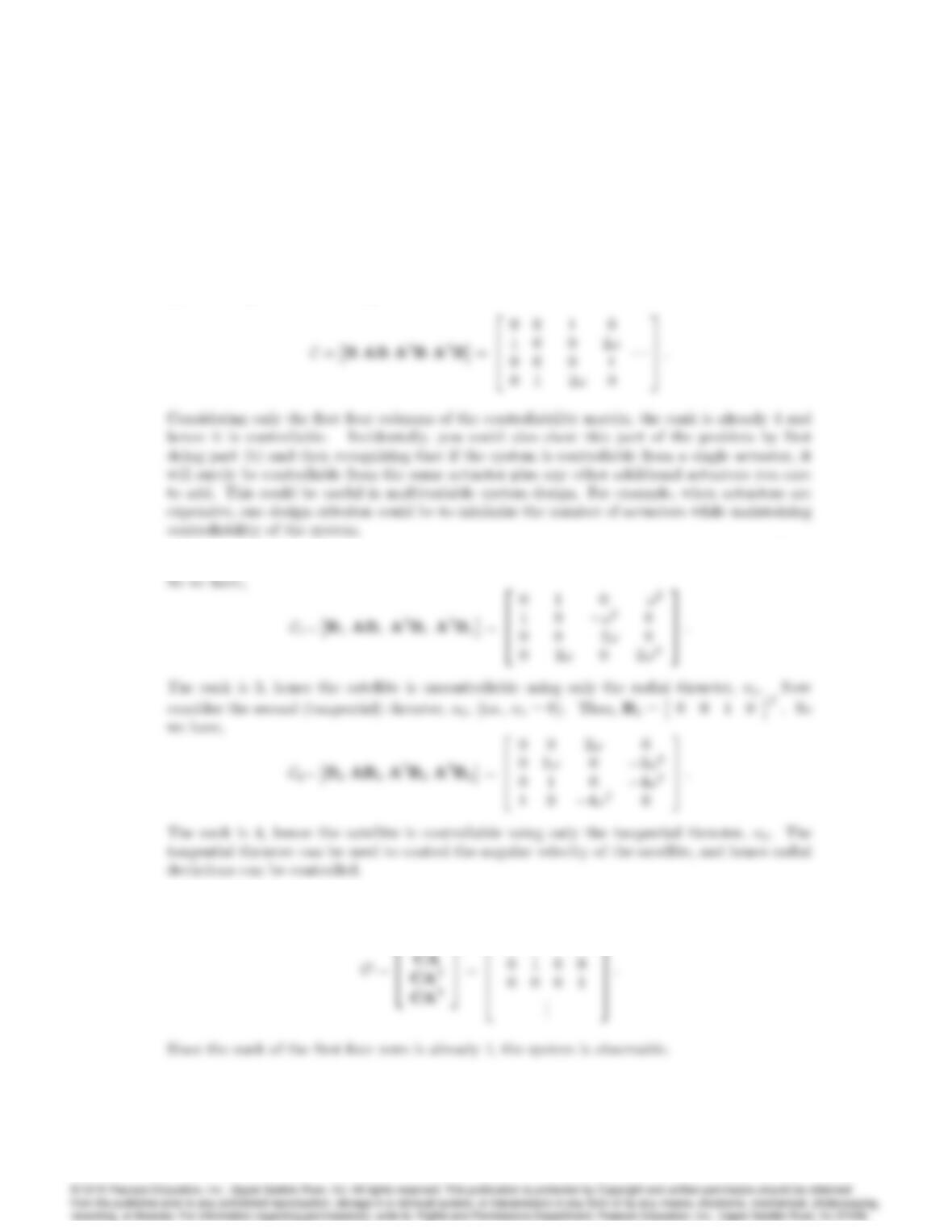
(a) Checking the controllability matrix:
(b) Consider only the first (radial) thruster, u1, (i.e., u2= 0). Then B1=0100T:
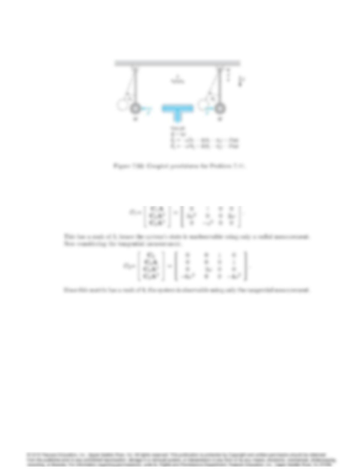
(c) Checking the observability matrix:
C
3
6
1000
0010
3
7
7050 CHAPTER 7. STATE-SPACE DESIGN
(d) Using only the first measurement, y1, we have,
C1
3
1 0 0 0
3
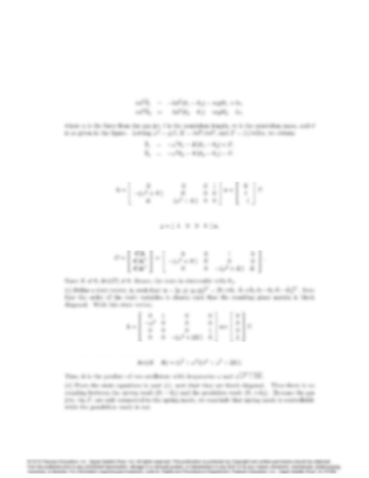
41. Consider the system in Fig. 7.93.
a) Write the state-variable equations for the system, using [12_
1_
2]Tas the state vector and
Fas the single input.
b) Show that all the state variables are observable using measurements of 1alone.
c) Show that the characteristic polynomial for the system is the product of the polynomials for
two oscillators. Do so by first writing a new set of system equations involving the state variables
2
6
6
4
y1
y2
_y1
_y2
3
7
7
5=2
6
6
4
1+2
12
_
1+_
2
_
1_
2
3
7
7
5:
Hint: If Aand Dare invertible matrices, then,
A 0
0 D 1
=A10
0 D1:
7051
d) Deduce the fact that the spring mode is controllable with Fbut the pendulum mode is not.
Solution:
The equations of motion for the system given in Fig. 7.93
(a) Using the state vector x= [12_
1_
2]T,
0 0 1 0
3
0
3
(b) Considering only the measurement of 1, then:
Observability:
C
3
1000
3
The characteristic equation of the system is,
7052 CHAPTER 7. STATE-SPACE DESIGN
42. A certain fifth-order system is found to have a characteristic equation with roots at 0, 1,2,
and 11j. A decomposition into controllable and uncontrollable parts discloses that the
controllable part has a characteristic equation with roots 0, and 11j. A decomposition into
observable and nonobservable parts discloses that the observable modes are at 0, 1, and 2.
a) Where are the zeros of b(s) = Cadj(sIA)Bfor this system?
b) What are the poles of the reduced-order transfer function that includes only controllable and
observable modes?
Solution:
(a) b(s) = Cadj(sIA)B
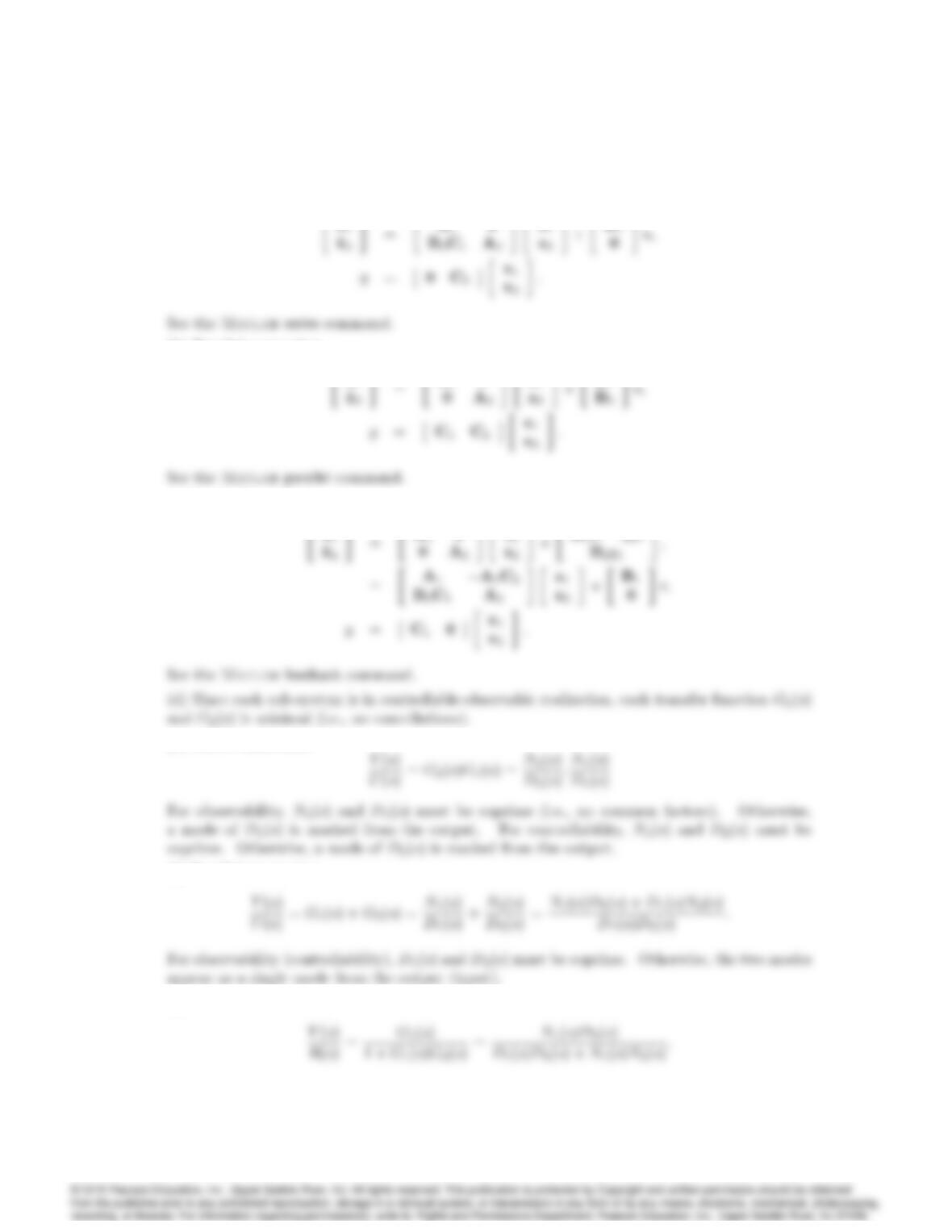
43. Consider the systems shown in Fig. 7.94, employing series, parallel, and feedback configurations.
a) Suppose we have controllable-observable realizations for each subsystem:
_
xi=Aixi+Biui;
yi=Cixi;where i= 1;2:
Give a set of state equations for the combined systems in Fig. 7.94.
b) For each case, determine what condition(s) on the roots of the polynomials Niand Diis
necessary for each system to be controllable and observable. Give a brief reason for your answer
in terms of pole-zero cancellations.
7053
Solution:
(a) Series connection,
_x1
(b) Parallel connection,
_x1
(c) Feedback connection,
_x1
(e) Series connection:
(f) Parallel connection:
(g) Feedback connection:
7054 CHAPTER 7. STATE-SPACE DESIGN
44. Consider the system •y+ 3 _y+ 2y= _u+u.
a) Find the state matrices Ac,Bc, and Ccin control canonical form that correspond to the
given differential equation.
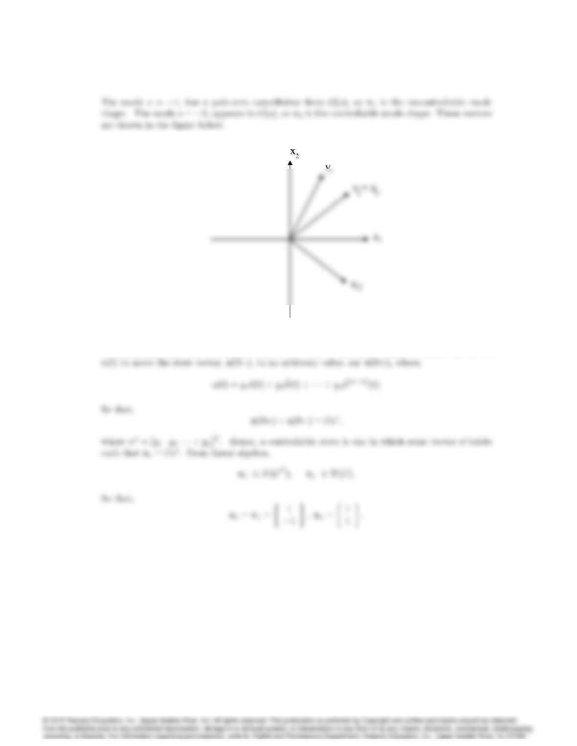
b) Sketch the eigenvectors of Acin the (x1; x2)plane, and draw vectors that correspond to the
completely observable (x0)and the completely unobservable (x
0)state variables.
c) Express x0and x
0in terms of the observability matrix O.
d) Give the state matrices in observer canonical form and repeat parts (b) and (c) in terms of
controllability instead of observability.
Solution:
(a) The Laplace transform of the differential equation gives the transfer function,
Hence in controller canonical form,
(b) First, we find the eigenvectors of Acor the modal directions of the system,
Using partial-fraction expansion of G(s), we can determine which modes are unobservable and
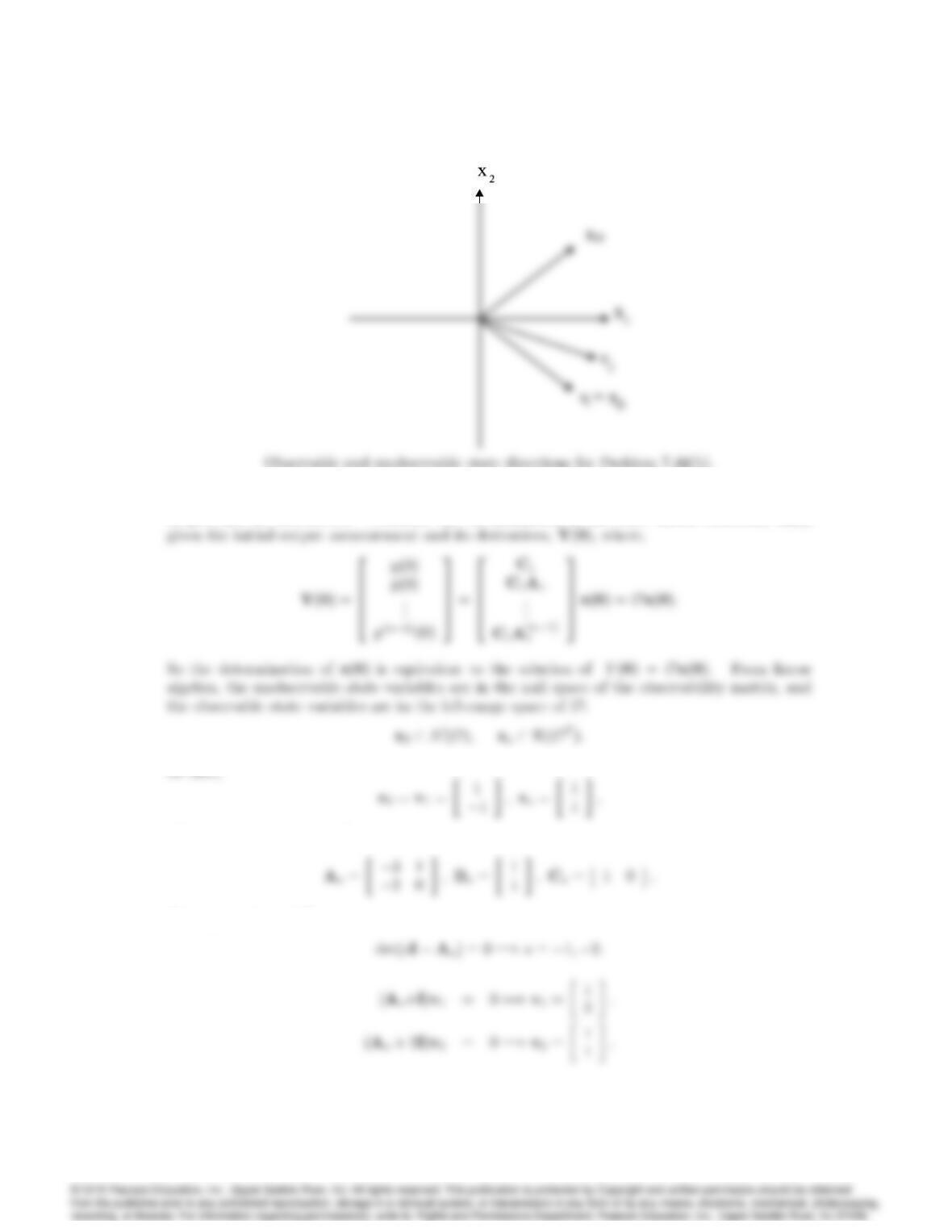
7055
Observable and unobservable state directions for Problem 7.44(b).
(c) Observability measures the ability to reconstruct the realization state variables given an
output and its derivatives. Consider the determination of the state initial condition, x(0),
(d) In observer canonical form,
The eigenvectors of Foare,
7056 CHAPTER 7. STATE-SPACE DESIGN
Controllable and uncontrollable state directions for Problem 7.44(d).
Controllability measures the ability to drive the states to arbitrary values. Consider the use of
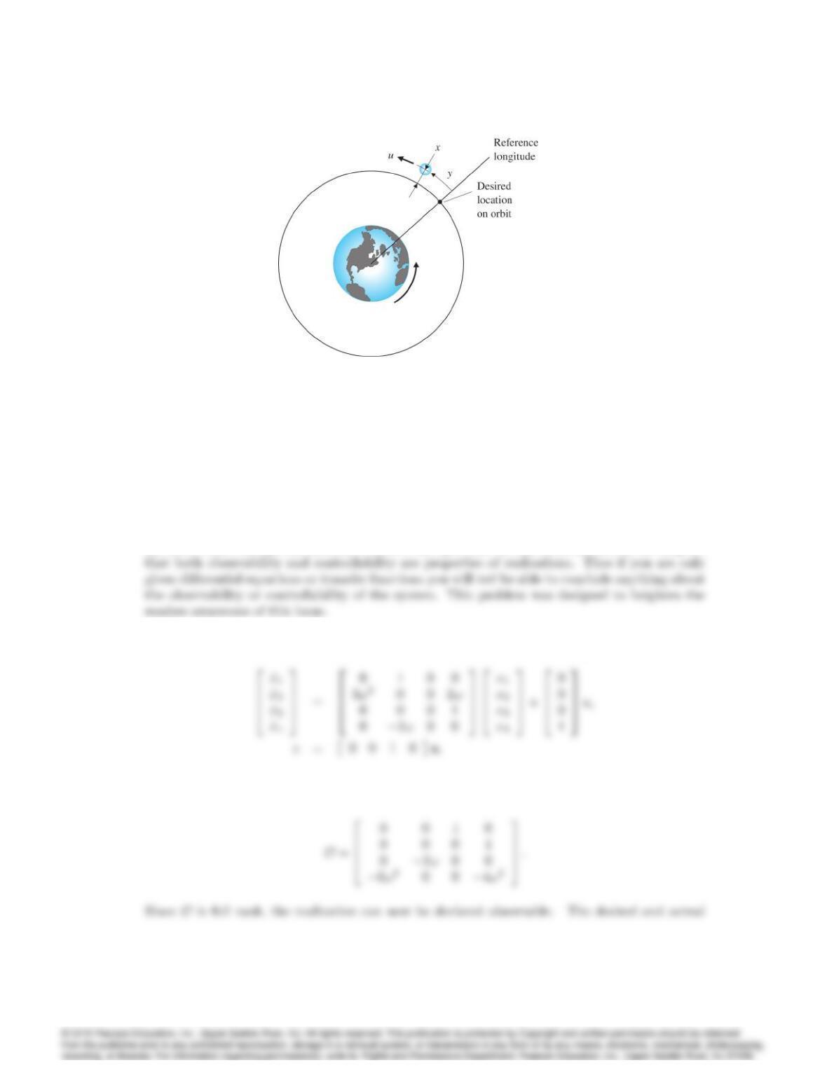
45. The equations of motion for a station-keeping satellite (such as a weather satellite) are
•x2!_y3!2x= 0;•y+ 2!_x=u;
where,
x= radial perturbation;
y= longitudinal position perturbation;
u= engine thrust in the y direction;
7057
Figure 7.95: Diagram of a station-keeping satellite in orbit for Problem 7.45.
as depicted in Fig. 7.94. If the orbit is synchronous with the earth’s rotation, then !=
2=(3600 24) rad/sec.
a) Is the state [x_x y _y]Tobservable?
b) Choose x= [ x_x y _y]Tas the state vector and yas the measurement, and design a
full-order observer with poles placed at s=2!,3!, and 3!3!j.
Solution:
(a) There is not enough information to answer this question. Recall, as mentioned in the chapter,
(b) Choosing x1=x,x2= _x,x3=y,x4= _y, and zas the output of the system (so that it
doesn’t conflict with the variable y, we have the following in state space equations.
Now that we have a realization for the system, we can check the observability to verify that we
can arbitrarily place the estimator poles. The observability matrix is,
7058 CHAPTER 7. STATE-SPACE DESIGN
estimator characteristic equations are,
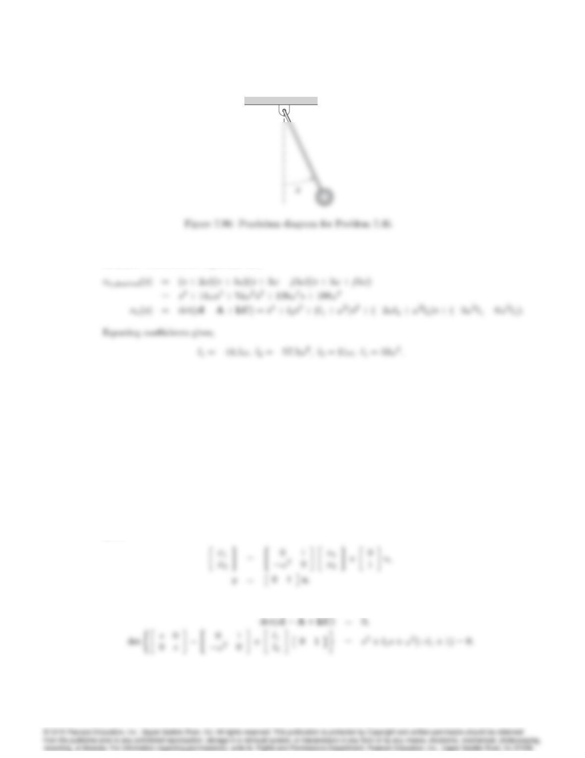
46. The linearized equations of motion of the simple pendulum in Fig. 7.96 are
•
+!2=u:
a) Write the equations of motion in state-space form.
b) Design an estimator (observer) that reconstructs the state of the pendulum given measure-
ments of _
. Assume != 5 rad/sec, and pick the estimator roots to be at s=10 10j.
c) Write the transfer function of the estimator between the measured value of _
and the esti-
mated value of .
d) Design a controller (that is, determine the state feedback gain K) so that the roots of the
closed-loop characteristic equation are at s=44j.
Solution:
(a) Defining x1=and x2=_
, and anticipating that the measured variable in part (b) is _
, we
have,
(b) From,
7059
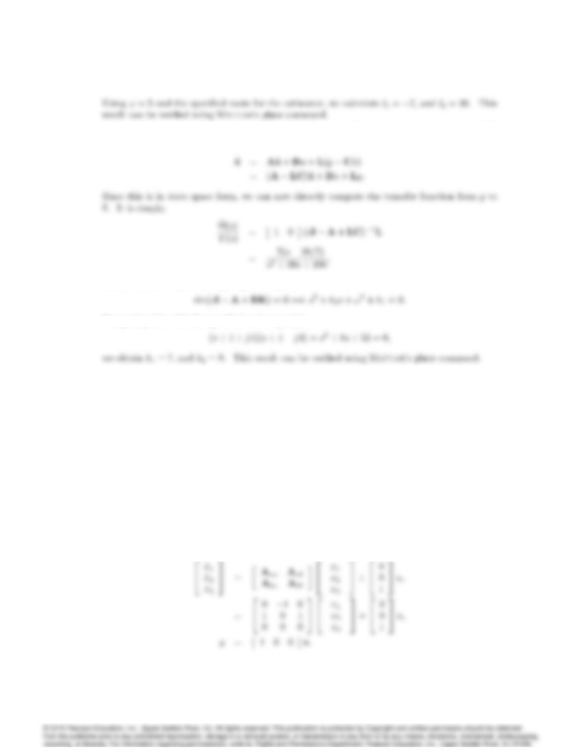
(c) To find the transfer function from the measured value of _
,y, to the estimated value of ,^
,
we use the estimator equations,
(d) For controller gain K= [k1k2], we require,
Comparing this with the specified roots equation:
47. An error analysis of an inertial navigator leads to the set of normalized state equations
2
4
_x1
_x2
_x33
5=2
4
01 0
1 0 1
0 0 0 3
52
4
x1
x2
x33
5+2
4
0
0
13
5u;
where
x1= east velocity error;
x2= platform tilt about the north axis;
x3= north gyro drift;
u= gyro drift rate of change:
Design a reduced-order estimator with y=x1as the measurement, and place the observer error
poles at 0:1and 0:1. Be sure to provide all the relevant estimator equations.
Solution:
Partitioning the system matrices yields,