7100 CHAPTER 7. STATE-SPACE DESIGN
10
-1
10
0
10
1
10
2
0
45
Bode D iag ram
Frequency (rad/sec)
10
-1
10
0
10
1
10
2
0
45
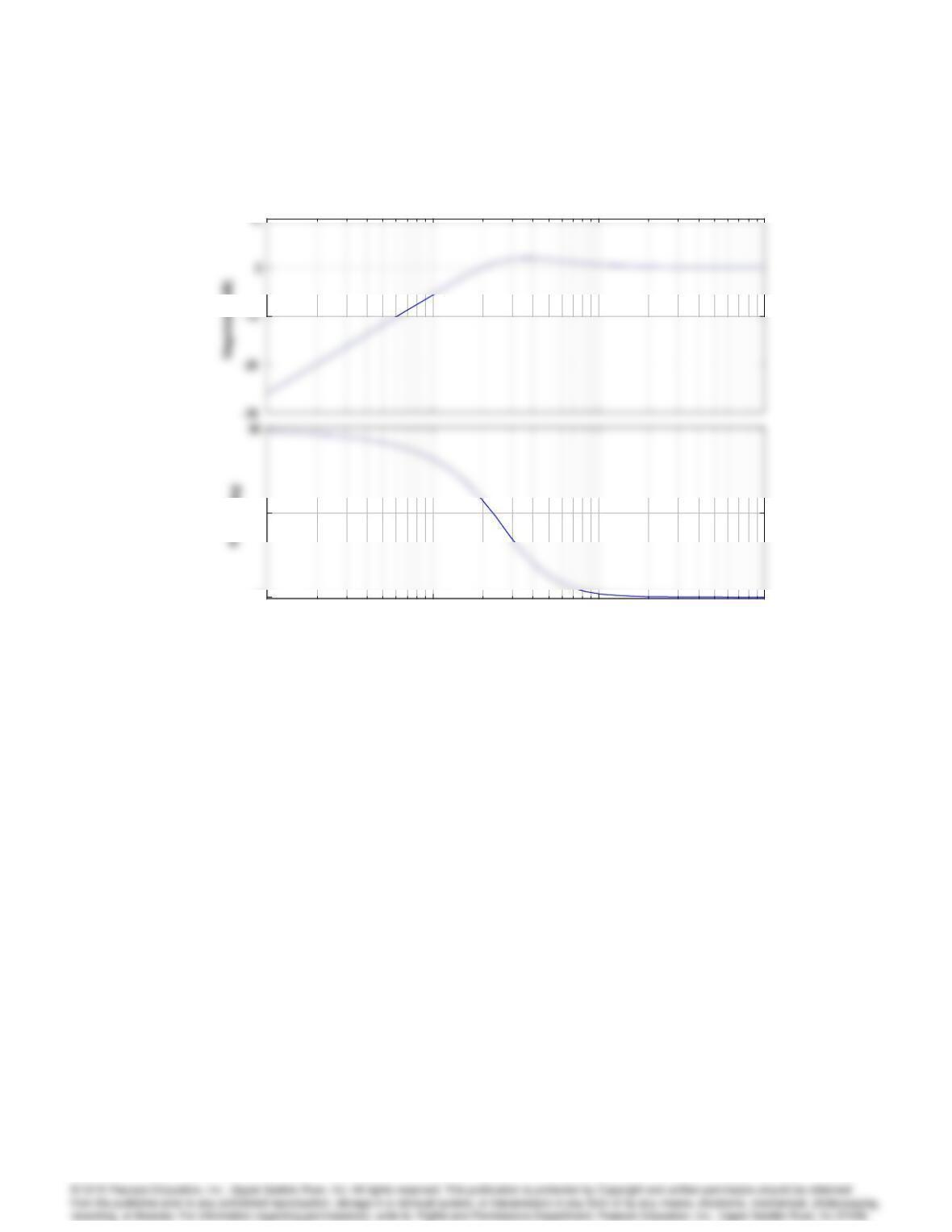
Bode plot of the sensitivity function for roblem 7.58.
59. NConsider a servomechanism for following the data track on a computer-disk memory system.
Because of various unavoidable mechanical imperfections, the data track is not exactly a centered
circle, and thus the radial servo must follow a sinusoidal input of radian frequency !0(the spin
rate of the disk). The state matrices for a linearized model of such a system are
A=0 1
01;B=0
1;C= [ 1 0 ]:
The sinusoidal reference input satisfies •r=!2
0r.
a) Let !0= 1, and place the poles of the error system for an internal model design at,
c(s) = (s+ 2 j2)(s+ 1 1j);
and the pole of the reduced-order estimator at
e(s) = (s+ 6):
b) Draw a block diagram of the system, and clearly show the presence of the oscillator with
frequency !0(the internal model) in the controller. Also verify the presence of the blocking
7101
–80
–60
–40
–20
0
20
Magnitude ( dB)
10
-1
10
0
10
1
10
2
–180
–135
–90
–45
0
Phase (deg)
Bode D iag ram
Frequency (rad/sec)
–80
–60
–40
–20
0
20
Magnitude ( dB)
10
-1
10
0
10
1
10
2
–180
–135
–90
–45
0
Phase (deg)
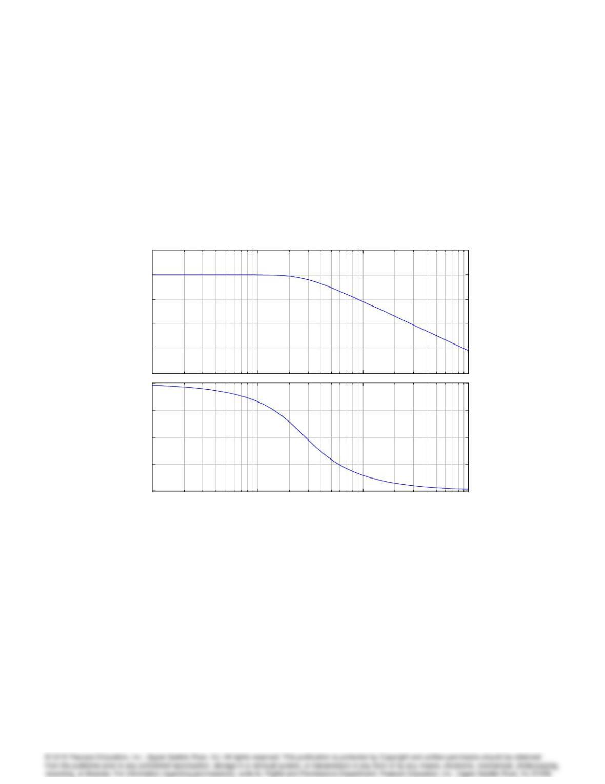
Figure 7.102: Bode plot of the complementary sensitivity function for Problem 7.58.
7102 CHAPTER 7. STATE-SPACE DESIGN
zeros at j!0.
c) Use Matlab (Simulink) software to plot the time response of the system to a sinusoidal input
at frequency !0= 1.
d) Draw a Bode plot to show how this system will respond to sinusoidal inputs at frequencies
different from but near !0.
Solution:
(a) The compensator design consists of two parts: a feedback design using an internal model
approach, and a reduced-order estimator. Let xbe the plant state vector where,
with,
e
3
0 1 0 0
3
0
3
when s=2j2;1j1, for,
So that the equation for the estimate of only x2is,
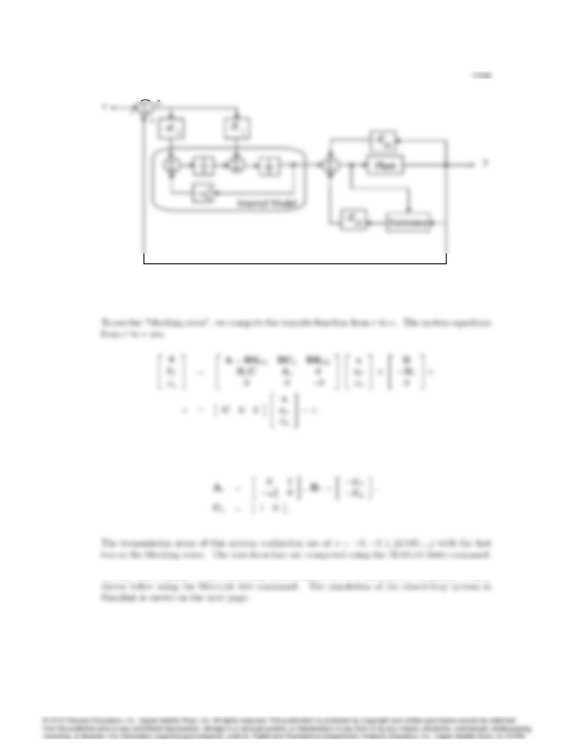
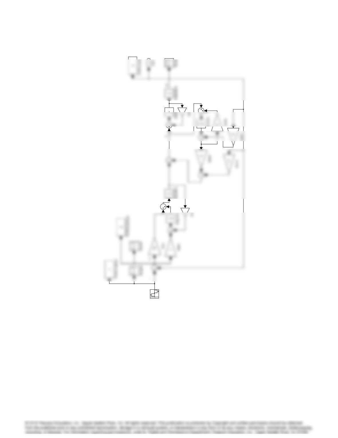
Problem 7.59: Compensator structure for robust following of sinusoid using an internal model
controller and reduced-order estimator.
where,
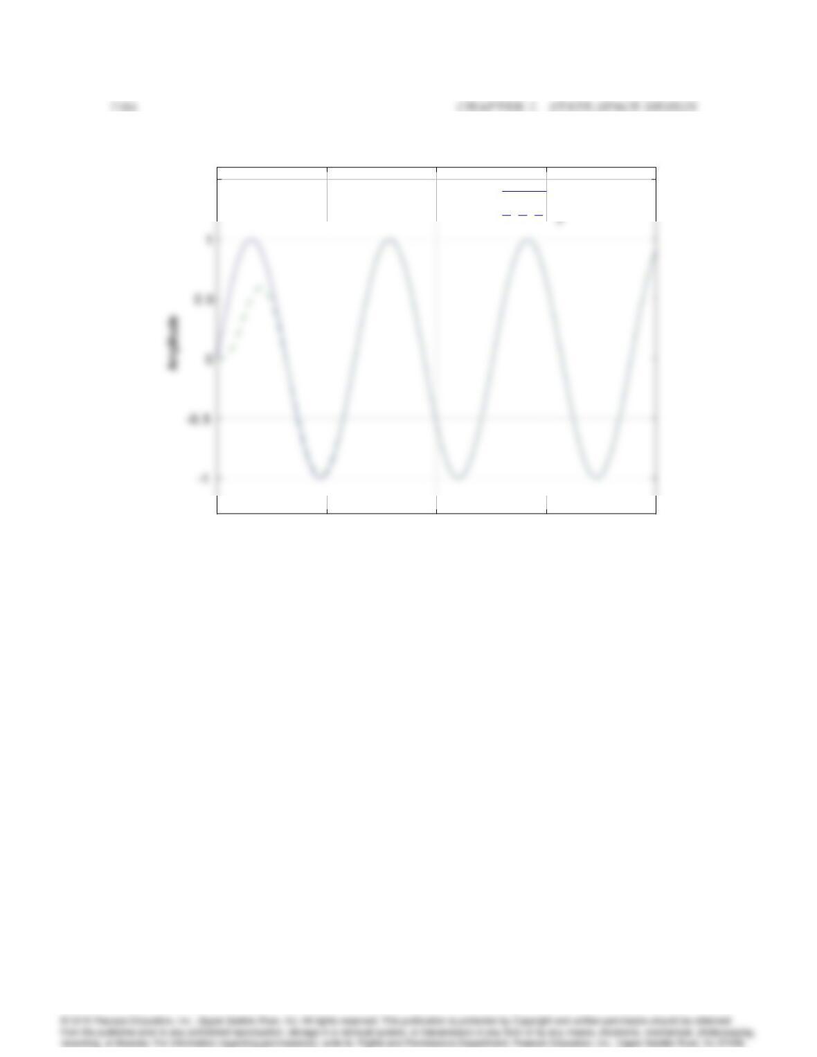
(c) The time response of the closed-loop system subjected to a sinusoid at a frequency of !0is
0 5 10 15 20
1.5
Time (sec)
r
y
0 5 10 15 20
1.5
Time (sec)
r
y
Problem 7.59: Time history of closed-loop system with a sinusoidial input.
7105
Sine Wave
Integrator4
Integrator1
-6
Simulink simulation for Problem 7.59.
7106 CHAPTER 7. STATE-SPACE DESIGN
–150
–50
50
–270
–90
Bode D iag ram
–150
–50
50
–270
–90
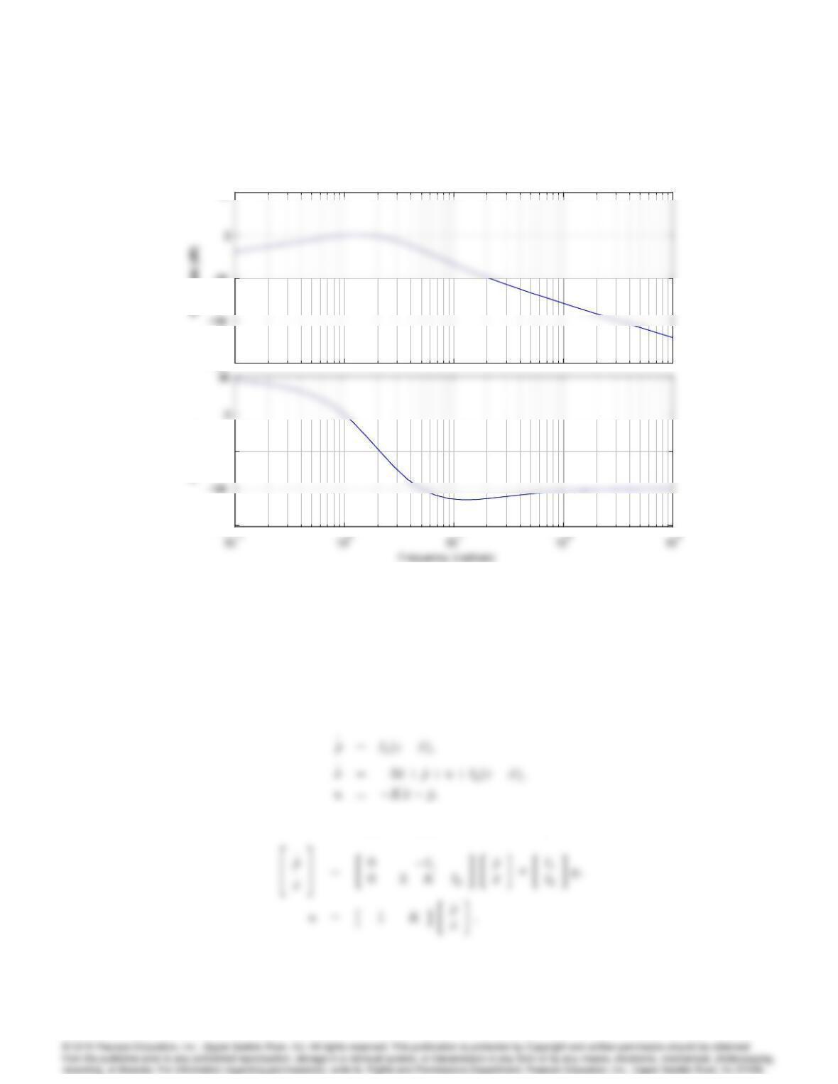
Problem 7.59: Bode plot of closed-loop system for sinusoidal following.
(d) A Bode plot of the compensated system is given above.
60. NCompute the controller transfer function (from Y(s)to U(s)) in Example 7.38. What is the
prominent feature of the controller that allows tracking and disturbance rejection?
Solution:
The related equations from the Text are,
To find the transfer function from Y(s)to U(s), we re-write the equations as,
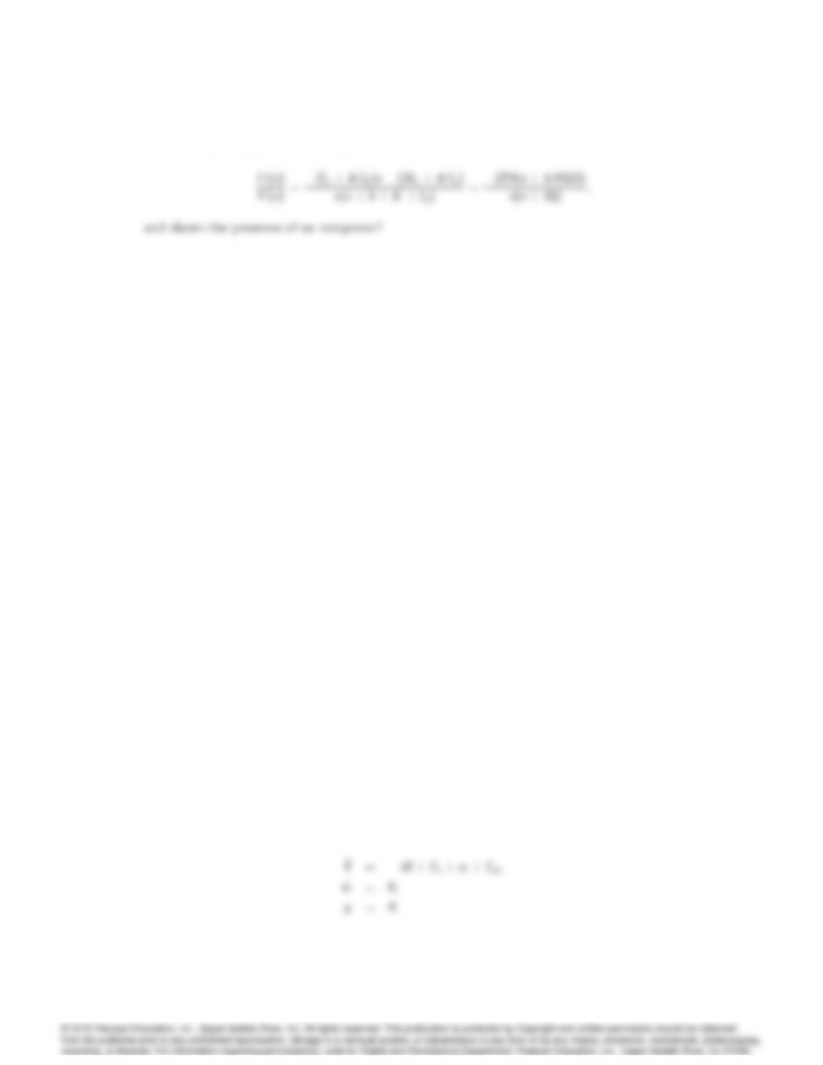
7107
The controller transfer function is,
61. NConsider the pendulum problem with control torque Tcand disturbance torque Td:
•
+ 4=Tc+Td;
(here g=l = 4.) Assume that there is a potentiometer at the pin that measures the output angle
, but with a constant unknown bias b. Thus the measurement equation is y=+b.
a) Take the “augmented” state vector to be
2
4
_
w3
5;
where wis the input-equivalent bias. Write the system equations in state-space form. Give
values for the matrices A,B, and C:
b) Using state-variable methods, show that the characteristic equation of the model is s(s2+4) =
0.
c) Show that wis observable if we assume that y=, and write the estimator equations for
2
6
4
^
_
^
^w
3
7
5:
Pick estimator gains [l1l2l3]Tto place all the roots of the estimator-error characteristic
equation at 10.
d) Using full-state feedback of the estimated (controllable) state-variables, derive a control law
to place the closed-loop poles at 22j.
e) Draw a block diagram of the complete closed-loop system (estimator, plant, and controller)
using integrator blocks.
f) Introduce the estimated bias into the control so as to yield zero steady-state error to the
output bias b. Demonstrate the performance of your design by plotting the response of the
system to a step change in b; that is, bchanges from 0 to some constant value.
Solution:
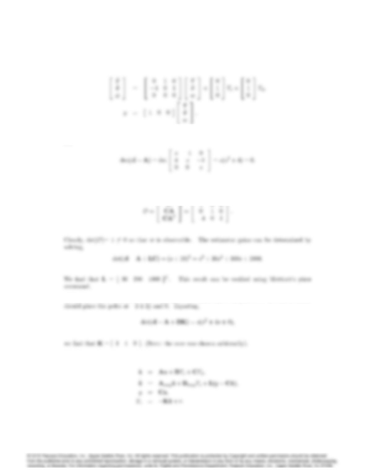
(a) The system with equivalent input disturbance which replaces the actual disturbance, b, with
the equivalent disturbance wat the control input is,
7108 CHAPTER 7. STATE-SPACE DESIGN
In state-space form,
(b)
(c) Forming the observability matrix, we have,
(d) The bias state variable wis not controllable, we cannot move the pole at 0. So state feedback
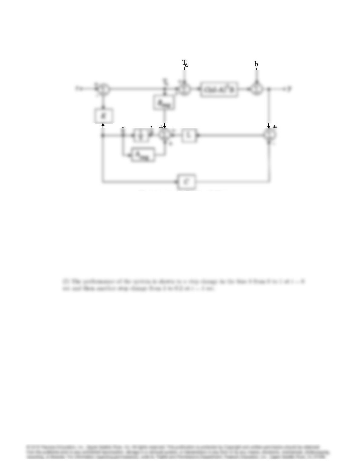
(e) The equations shown in the figure are,
7109
Block diagram for Problem 7.61(e).
7110 CHAPTER 7. STATE-SPACE DESIGN
-1
-1
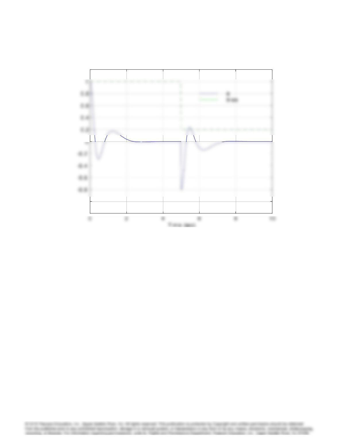
Problem 7.61: Step change in bias.
Problems for Section 7.10.3: Model-following Design
62. NConsider the servomechanism problem where we wish to track a ramp reference signal. The
plant and the desired model equations are
_x =0 1
01x+0
1u
y=1 0 x
_xm=0 1
0 0 xm
ym=1 0 xm
Design a model-following control law and demonstrate its tracking performance. Place the
closed-loop poles at s=2j2.
Solution:
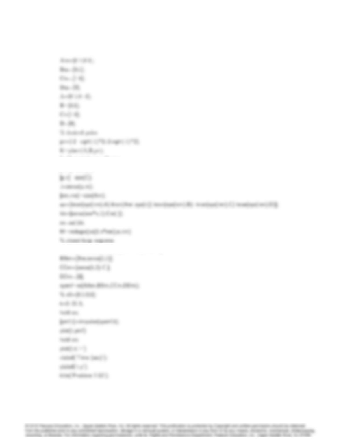
% Model-following Trankle & Bryson Example
% Reference Model
7111
% Model-following Design
[n,m]=size(B);
AAm=[Am zeros(2,2);B*(N+K*M) A-B*K];
7112 CHAPTER 7. STATE-SPACE DESIGN
nicegrid;
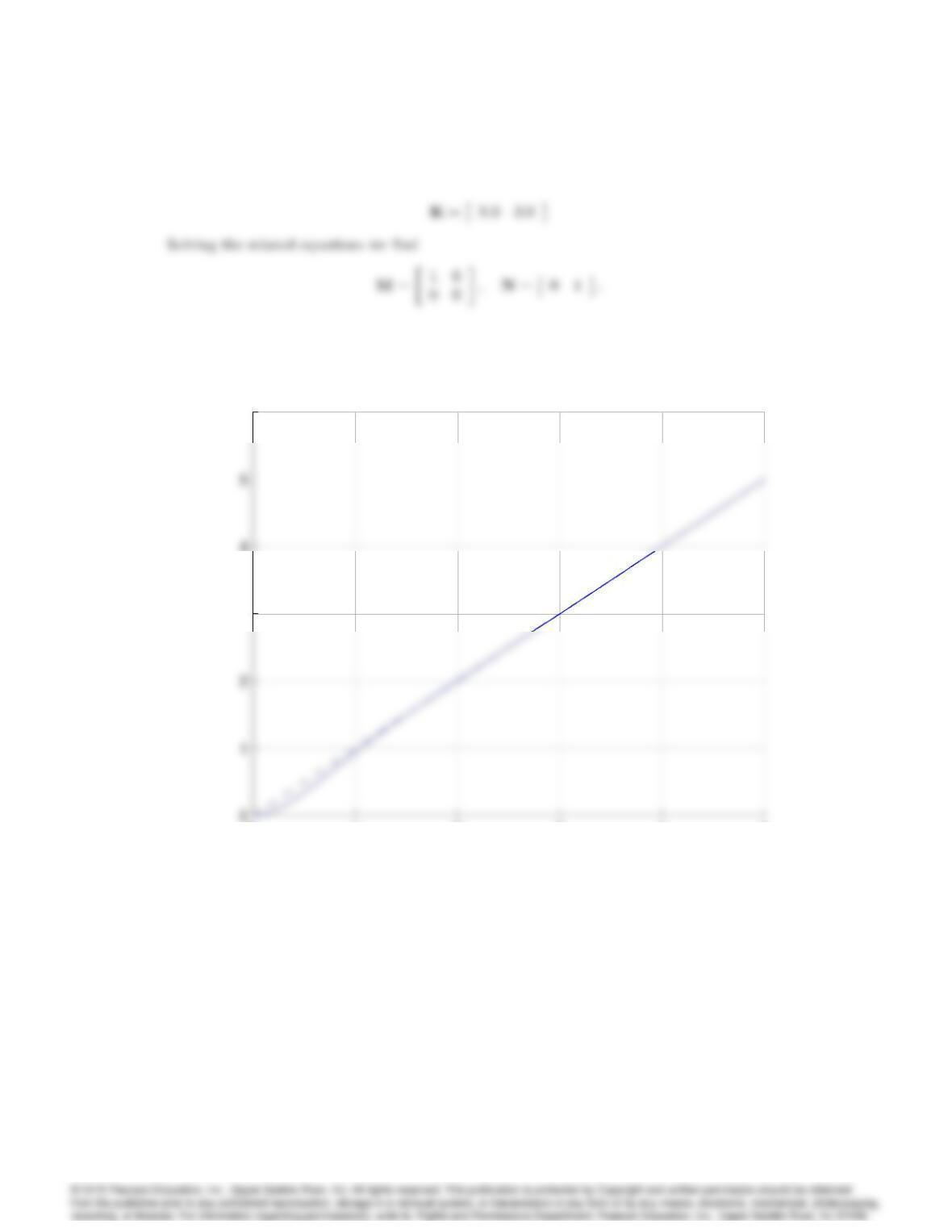
The response of the system is shown in the ensuing figure.
0 1 2 3 4 5
3
4
6
Time (sec)
r,y
0 1 2 3 4 5
3
4
6
Time (sec)
r,y
Model-following ramp response for Problem 7.62.
63. NImplicit Model-Following: Suppose we wish the closed-loop system to behave like a desired
model, called the implicit model
_z =Amz:
We may minimize a modified LQR performance index
J=
1
Z
0( _yAmy)TQ1( _yAmy) + uTRudt:
7113
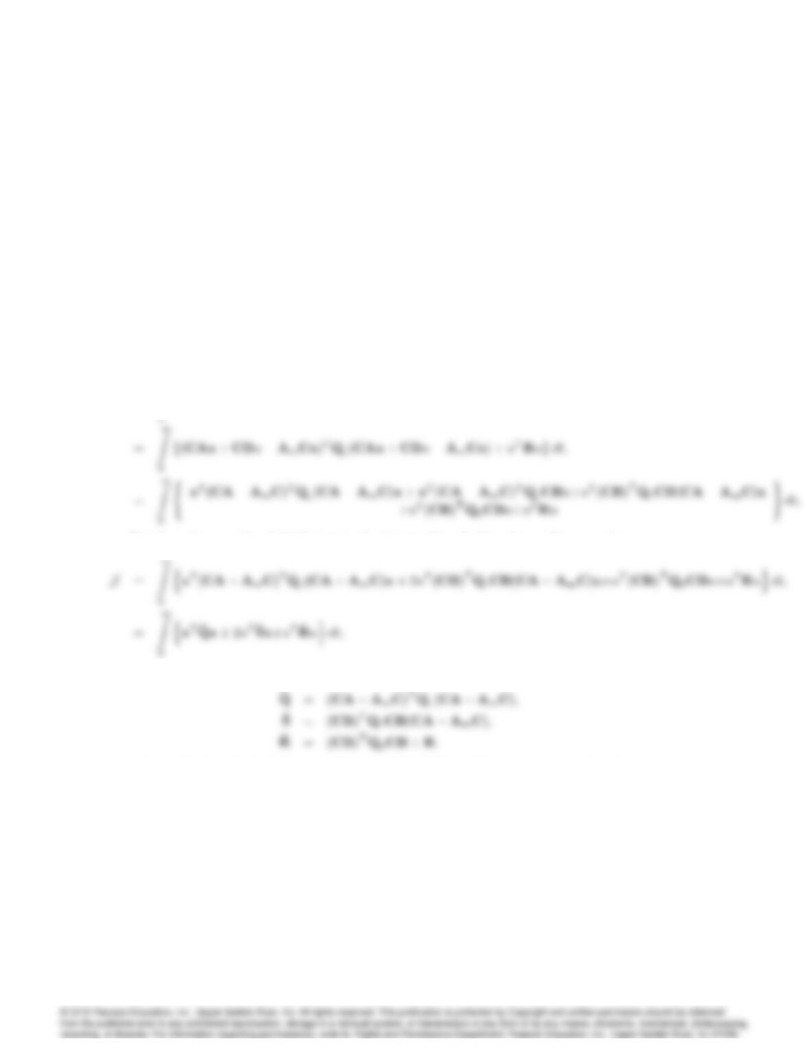
Show that this performance index is equivalent to the standard one with the addition of a
cross-weighting term between the control and the state of the form
J=
1
Z
0nxTb
Qx + 2uTb
Sx +uTb
Ruodt;
where
^
Q= (CA AmC)TQ1(CA AmC);
b
S=BTCTQ1(CA AmC);
b
R=R+BTCTQ1CB:
Solution:
J=
1
Z
But since the second and third term in the integrand are both scalars and are equal
where
1. 64. NExplicit Model-Following: Suppose in the LQR problem, we wish the closed-loop system
to behave as close as possible to a system of the form
_z =Amz;
which represents the model of desirable dynamics. We may choose a performance index of the
form
J=
1
Z
0(yz)TQ1(yz) + uTRudt:

7114 CHAPTER 7. STATE-SPACE DESIGN
(a) Show that this performance index can be converted to the standard one by augmenting the
states of the plant and the model i.e. choose the augmented state vector, =xTzTTand
write down the system equations to show that
J=
1
Z
0nTQ1+uTRuodt:
where
Q=CTQ1CCTQ1
Q1C Q1:
(b) Which states of the system are uncontrollable? Is this result surprising?
(c) The optimal control is of the form
u=K1xK2z;
which means that the model’s equations must be implemented as part of the control law. Suppose
we now drive the model as follows
_z =Amz+Bpup;
where upmay be the pilot input in an aircraft system. Show that
Y(s)
Up(s)=C(sIA+BK1)1
|{z }
Closedloop dynamics
K2(sIAm)1Bp
|{z }
F eedforward dynamics
:
This indicates that the feedforward dynamics may be used to improve the transient response of
the system.
(d) What are the transmission zeros of the overall system?
(e) What is a possible disadvantage of this scheme compared to the standard LQR, i.e., with no
explicit model?
Solution:
(a)
_
(b) The modes (eigenvalues) of Amare uncontrollable. No surprise as control does not affect those
modes.
7115
(c)
_
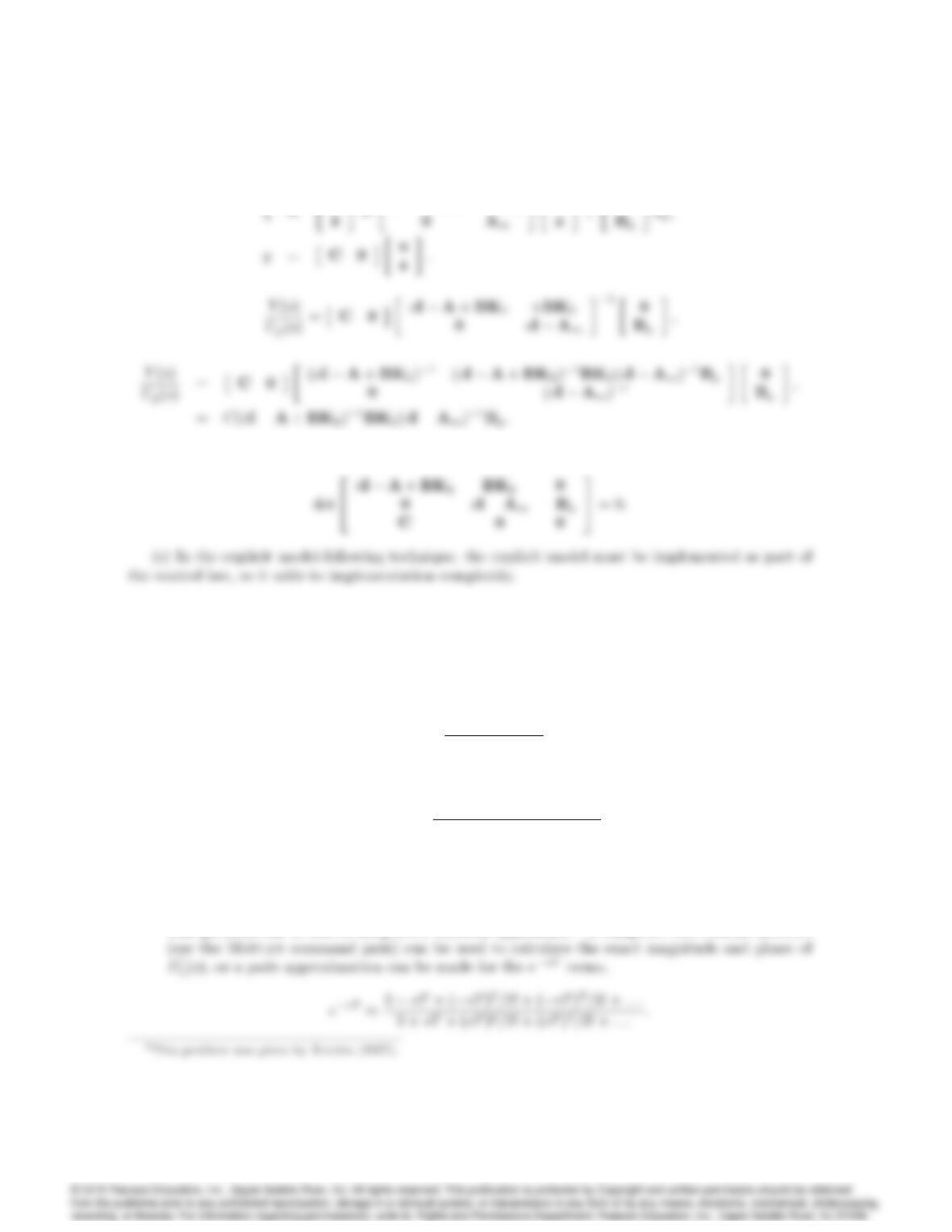
(d) The transmission zeros of the overall system are given by:
Problems for Section 7.13: Design for Systems with
Pure Time Delay
65. NConsider the system with the transfer function eT sG(s), where
G(s) = 1
s(s+ 1)(s+ 2):
1. The Smith compensator for this system is given by
D0
c(s) = Dc(s)
1 + (1 esT )G(s)Dc(s):
Plot the frequency response of the compensator for T= 5 and Dc(s) = 1, and draw a Bode plot
that shows the gain and phase margins of the system.2
Solution:
This problem can be solved using a few different approaches. A computer tool such as Matlab
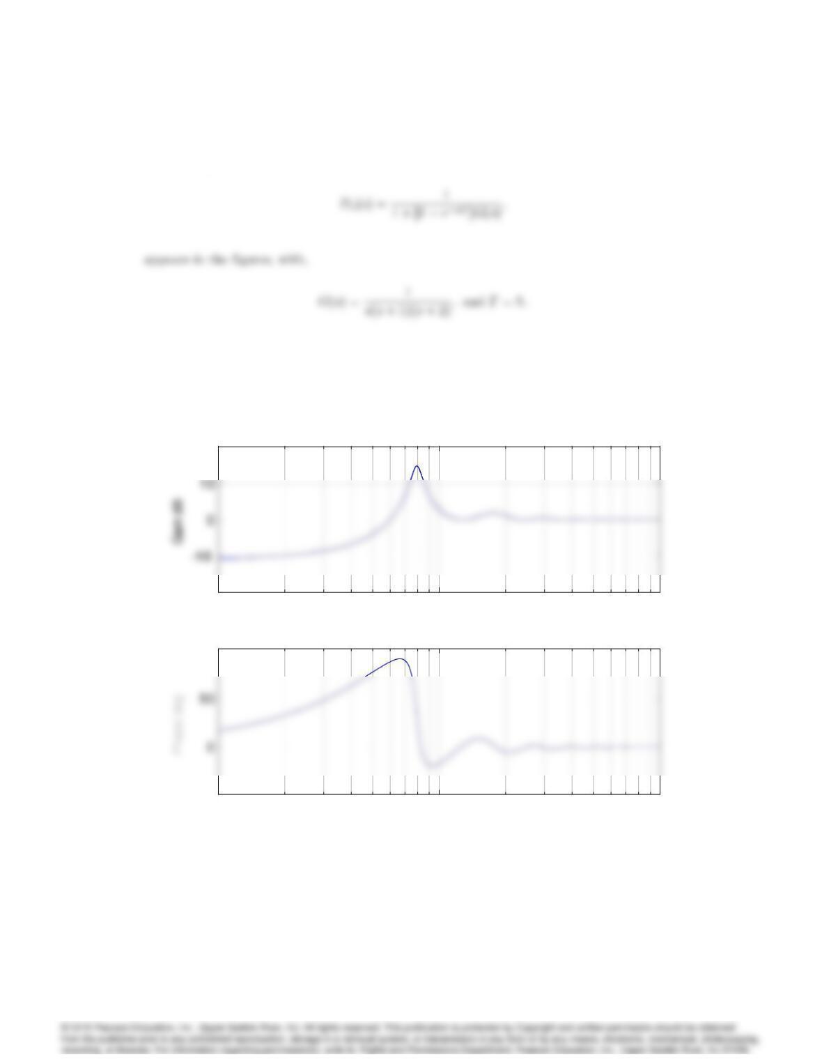
7116 CHAPTER 7. STATE-SPACE DESIGN
We will show both the exact calculation and Bode plots using a fourth-order pade approximation.
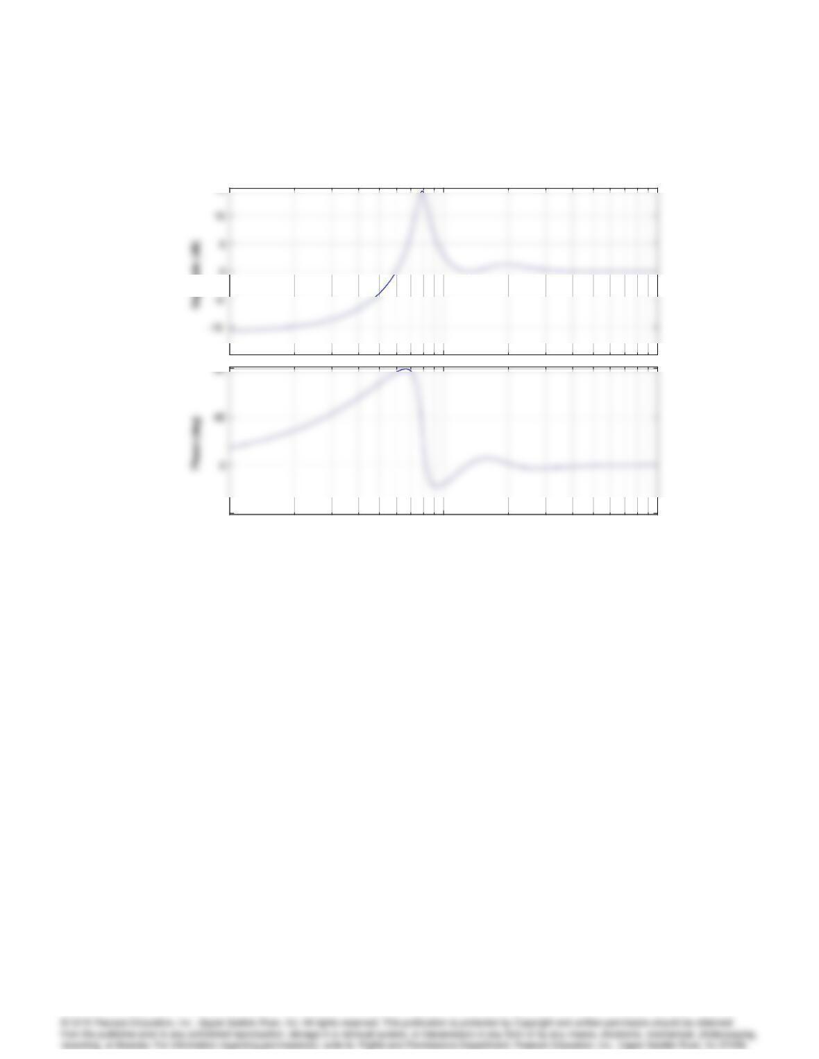
The Bode plot of the compensator
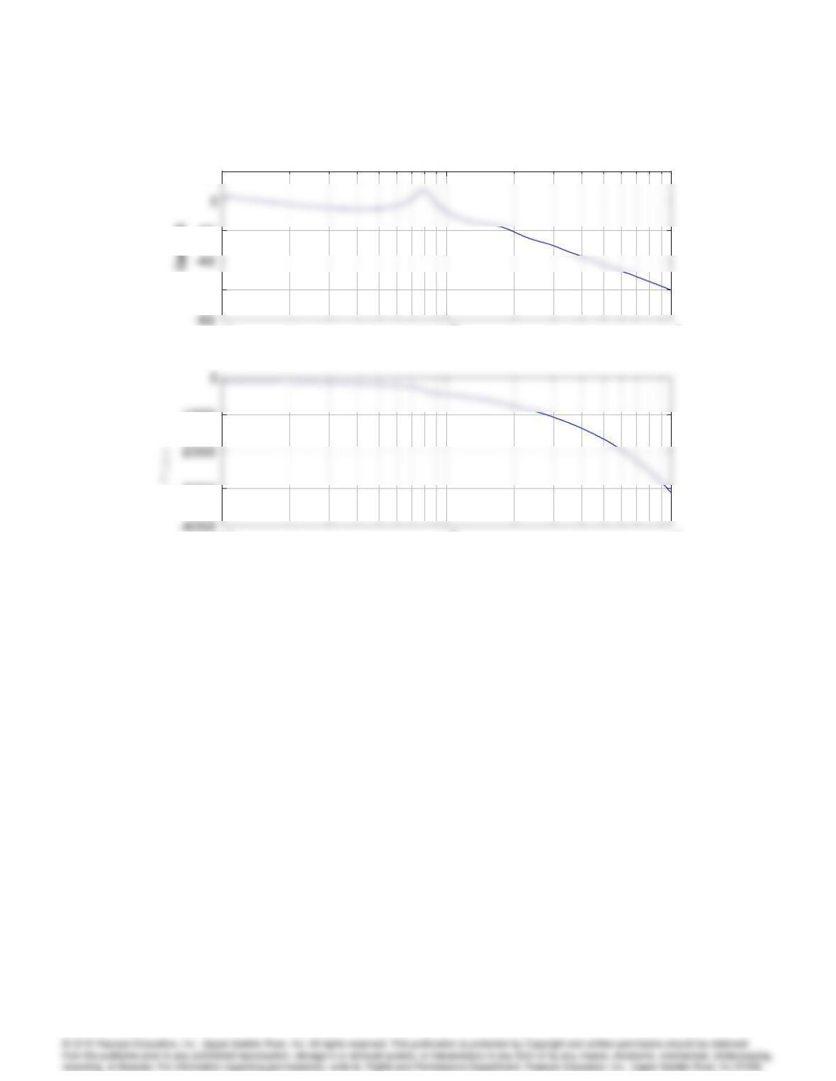
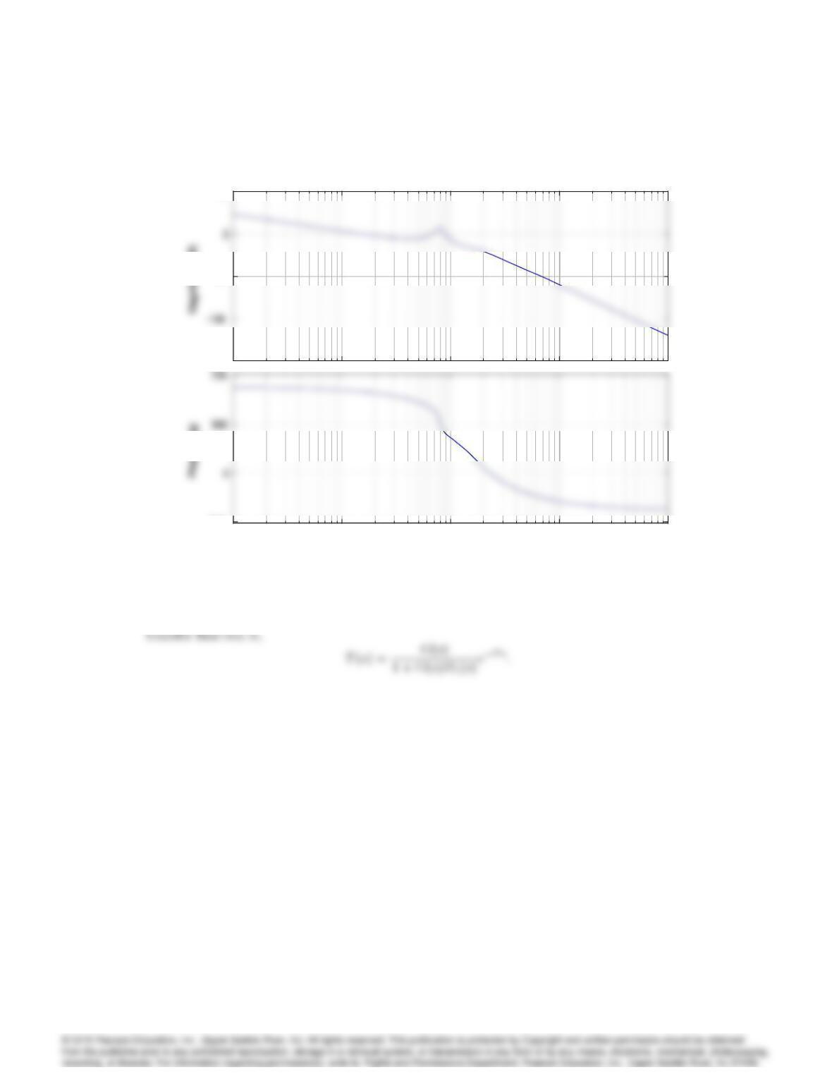
The Bode plot of the closed-loop system is also shown.
10-1 100101
–20
20
Frequency (rad/sec)
10-1 100101
–20
20
10-1 100101
–50
100
Frequency (rad/sec)
10-1 100101
–20
20
Frequency (rad/sec)
10-1 100101
–20
20
10-1 100101
–50
100
Problem 7.65 Bode plot of compensator D0
c(s): exact.
7117
–15
0
10
-1
10
0
10
1
–45
Bode D iag ram
Frequency (r ad/sec)
–15
0
10
-1
10
0
10
1
–45
Problem 7.65: Pade approximation.
7118 CHAPTER 7. STATE-SPACE DESIGN
10-1 100101
–3000
–1000
Frequency (rad/sec)
10-1 100101
–60
–20
20
Frequency (rad/sec)
10-1 100101
–3000
–1000
10-1 100101
–60
–20
20
Frequency (rad/sec)
Problem 7.65 Bode plot of closed-loop system: exact.
7119
–150
–50
50
10
-2
10
-1
10
0
10
1
10
2
–360
Bode D iag ram
Frequency (r ad/sec)
–150
–50
50
10
-2
10
-1
10
0
10
1
10
2
–360
Problem 7.65 Bode plot of closed-loop system: Pade approximation.
Remark: Note that the Smith compensator, D0
c(s), is structured such that the closed-loop