7080 CHAPTER 7. STATE-SPACE DESIGN
c) Could both state variables of the system be estimated if only a measurement of _ywas available?
d) Design a full-state feedback controller with roots at s=20 20j.
e) Would it be reasonable to design a control law for the system with roots at s=200 200j?
State your reasons.
f) Write equations for the compensator, including a command input for y. Draw a Bode plot
for the closed-loop system, and give the gain and phase margins for the design.
Solution:
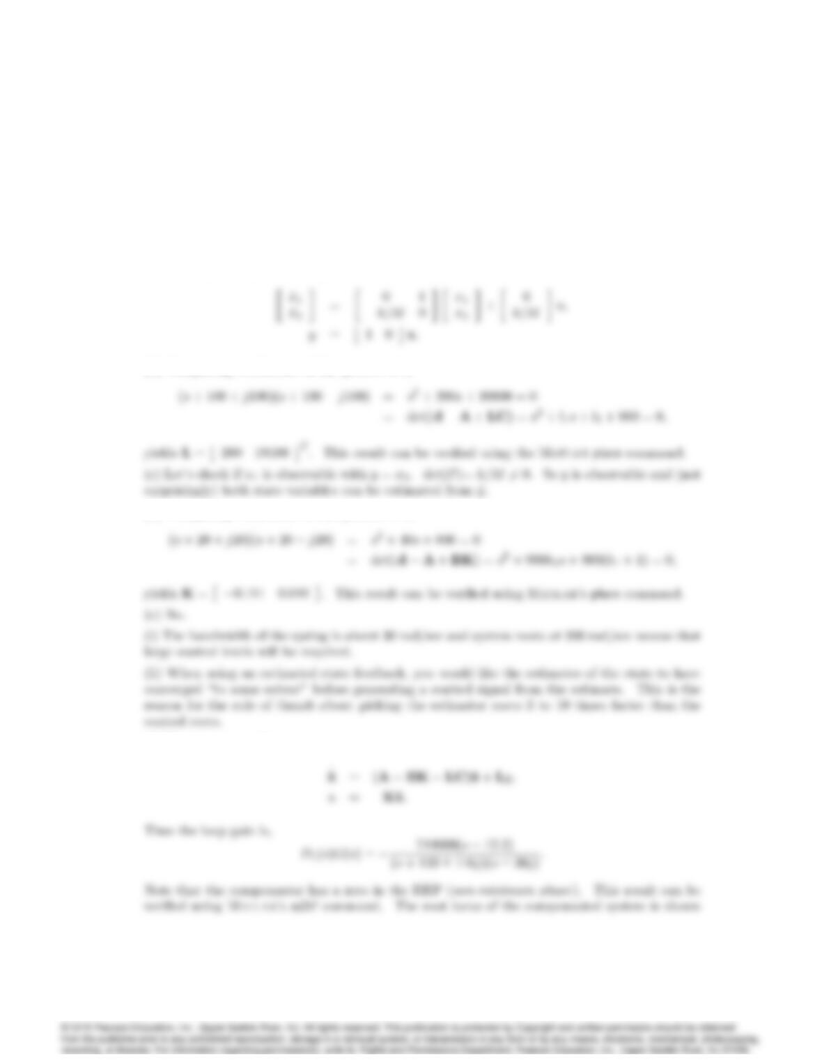
(a) Defining x1=yand x2= _y, we have,
(b) Comparing coe¢cients of like powers of s,
(d) Comparing coe¢cients of like powers of s,
(f) We can express the compensator as,
7081
Root Locus
Real Axis
-200 -150 -100 -50 050 100 150 200
-200
-50
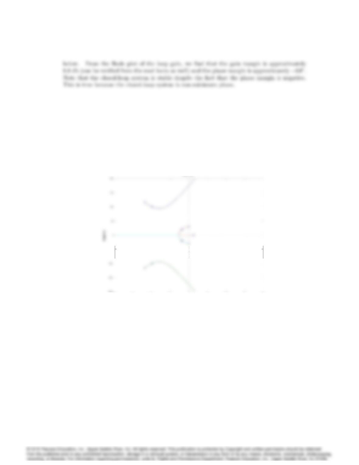
Root locus for Problem 7.53.
7082 CHAPTER 7. STATE-SPACE DESIGN
–100
10
-3
10
-2
10
-1
10
0
10
1
10
2
–270
Bode D iagram
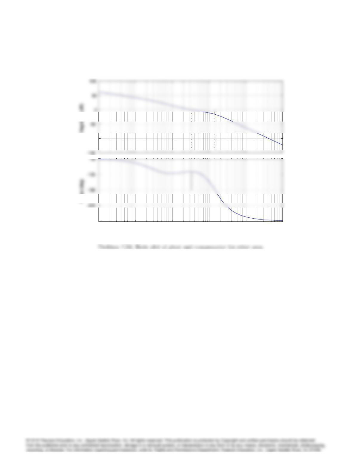
Gm = 15.8 dB (at 1.42 rad/sec) , Pm = 52.8 deg (at 0.334 rad/sec)
Frequency (rad/sec)
–100
10
-3
10
-2
10
-1
10
0
10
1
10
2
–270
54. The linearized di¤erential equations governing the ‡uid-‡ow dynamics for the two cascaded
tanks in Fig. 7.99 are
_
h1+h1=u;
_
h2+h2=h1;
where,
h1= deviation of depth in tank 1 from the nominal level;
h2= deviation of depth in tank 2 from the nominal level;
u = deviation in uid inow rate to tank 1 (control):
a) Level Controller for Two Cascaded Tanks: Using state feedback of the form,
u =K1h1K2h2;
choose values of K1and K2that will place the closed-loop eigenvalues at,
s=2(1 j):
7083
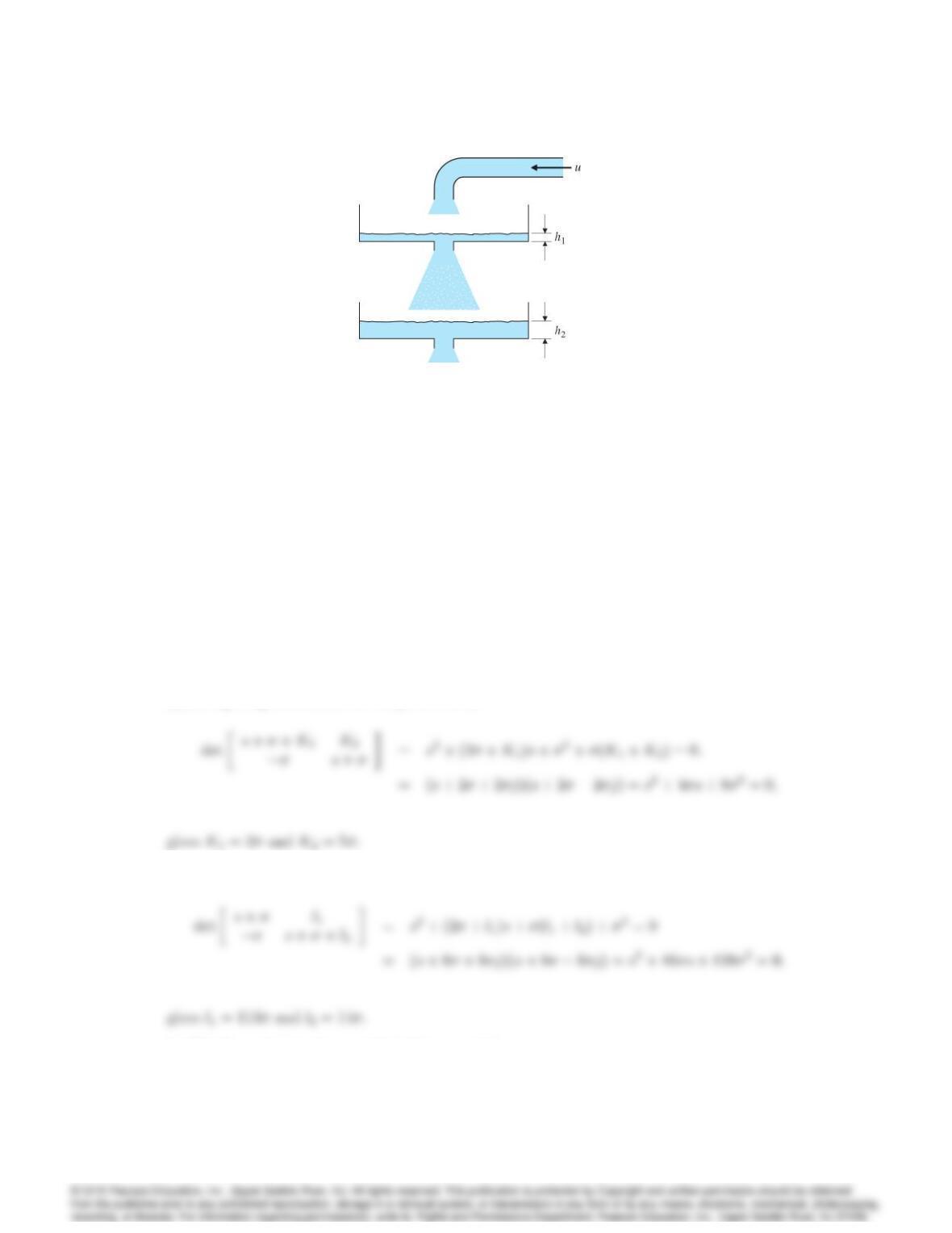
Figure 7.99: Coupled tanks for Problem 7.54.
b) Level Estimator for two Cascaded Tanks: Suppose that only the deviation in the level of
tank 2 is measured (that is, y=h2). Using this measurement, design an estimator that will
give continuous, smooth estimates of the deviation in levels of tank 1 and tank 2, with estimator
error poles at 8(1 j).
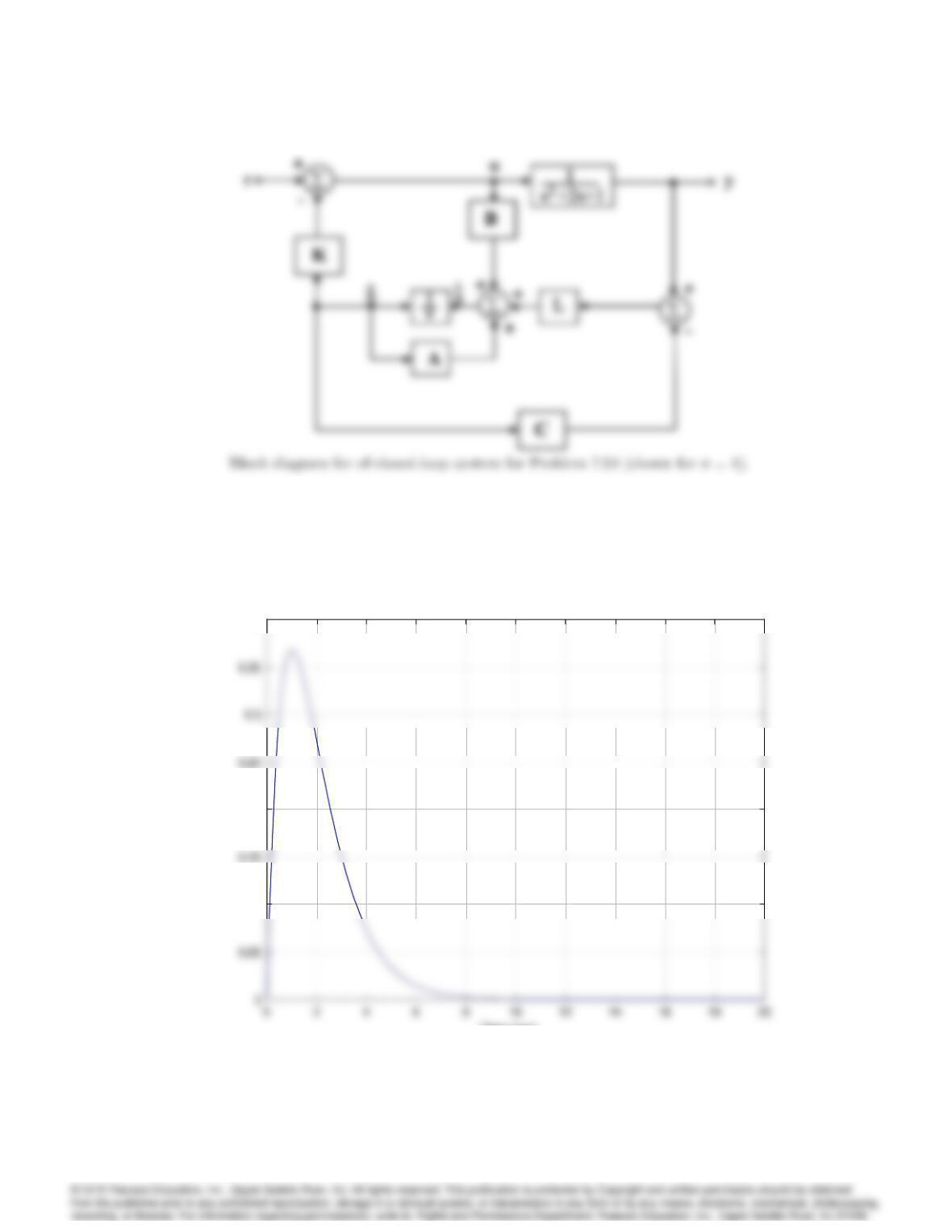
c) Estimator/Controller for Two Cascaded Tanks: Sketch a block diagram (showing individual
integrators) of the closed-loop system obtained by combining the estimator of part (b) with the
controller of part (a).
d) Using Matlab, compute and plot the response at yto an initial o¤set in h1. Assume = 1
for the plot.
Solution:
(a) Comparing coe¢cients of like powers of s,
(b) Comparing coe¢cients of like powers of s,
(c) The figure below shows a block diagram of the system.
7084 CHAPTER 7. STATE-SPACE DESIGN
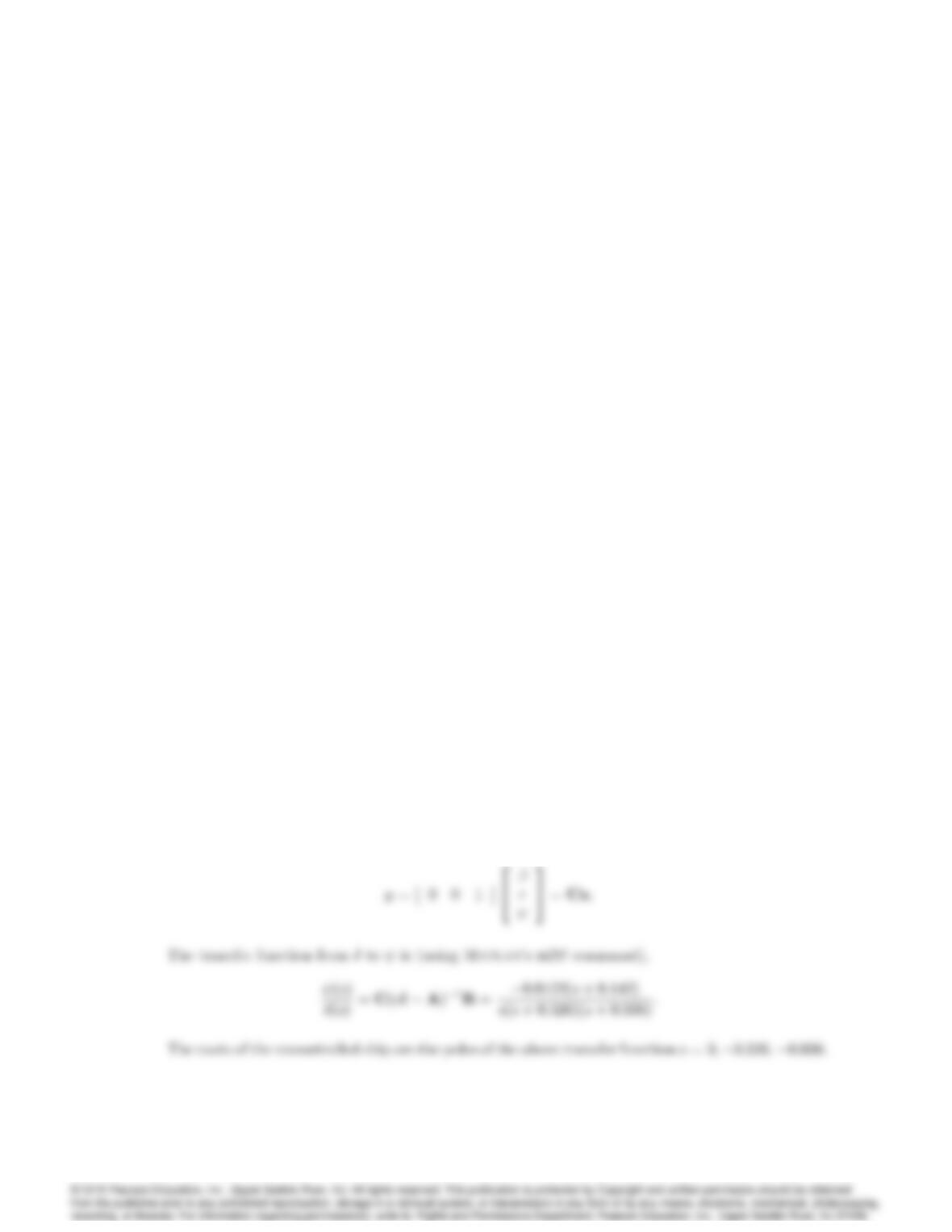
(d) The response to an initial condition on h1(0) is shown next using the Matlab initial
command.
0.1
0.2
0.4
Response to Initial Conditions
Time (sec)
Amplitude
0.1
0.2
0.4
7085
Problem 7.54: Initial condition response for o¤set in h1(0).
55. The lateral motions of a ship that is 100 m long, moving at a constant velocity of 10 m/sec, are
described by
2
4
_
_r
_
3
5=2
40:0895 0:286 0
0:0439 0:272 0
0 1 0
3
52
4
r
3
5+2
4
0:0145
0:0122
0
3
5;
where
= sideslip angle;deg;
= heading angle;
= rudder angle;deg;
r= yaw rate:See Fig:7:100:
a) Determine the transfer function from to and the characteristic roots of the uncon-
trolled ship.
b) Using complete state feedback of the form,
=K1K2rK3( d);
where dis the desired heading, determine values of K1,K2, and K3that will place the closed-
loop roots at s=0:2;0:20:2j.
c) Design a state estimator based on the measurement of (obtained from a gyrocompass, for
example). Place the roots of the estimator error equation at s=0:8and 0:80:8j.
d) Give the state equations and transfer function for the compensator Dc(s)in Fig. 7.101, and
plot its frequency response.
e) Draw the Bode plot for the closed-loop system, and compute the corresponding gain and
phase margins.
f) Compute the feed-forward gains for a reference input, and plot the step response of the system
to a change in heading of 5.
Solution:
(a) With as the measurement,
7086 CHAPTER 7. STATE-SPACE DESIGN
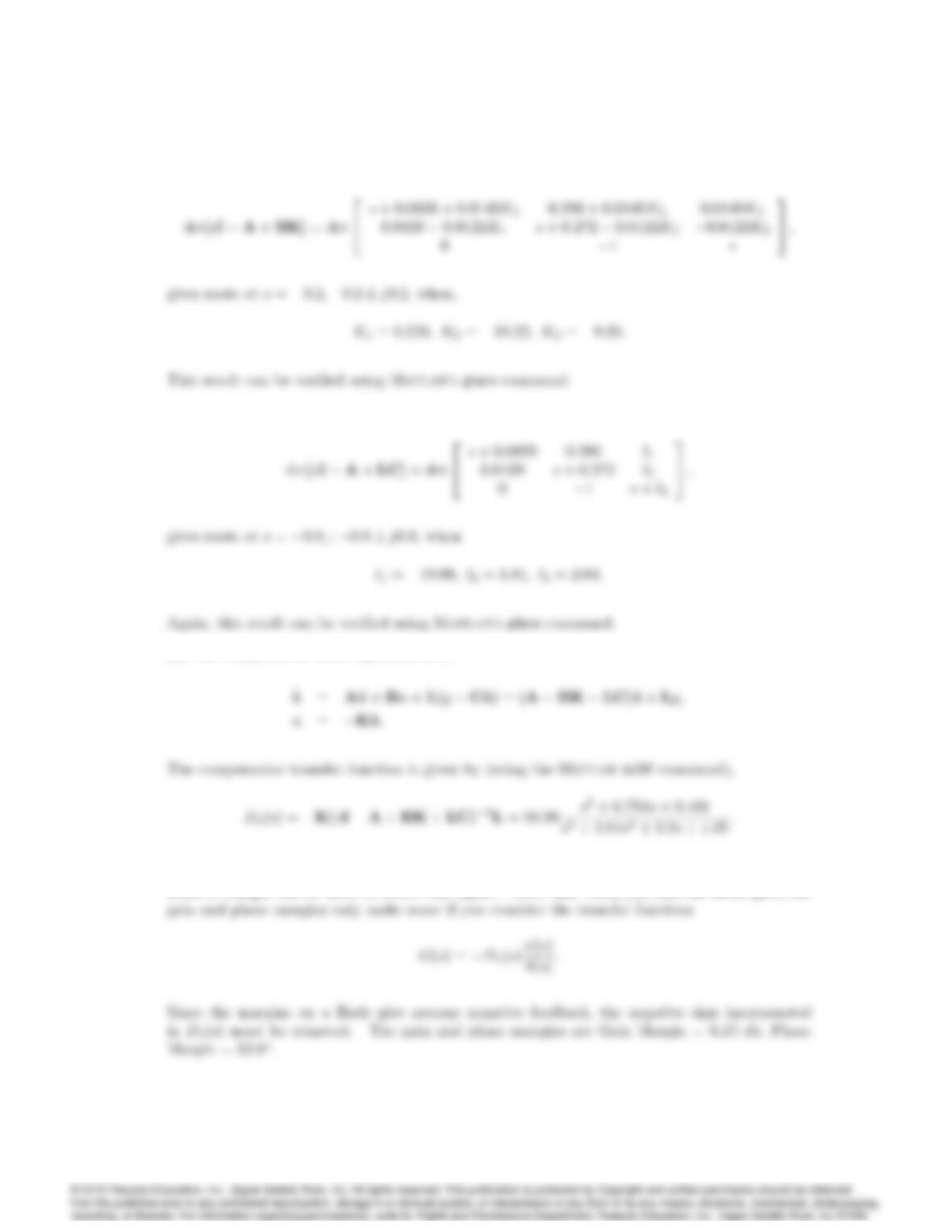
Figure 7.100: View of ship from above for Problem 7.55.
7087
(b) Define K=K1K2K3and let =Kx. Then,
(c) With L=l1l2l3T,
(d) The compensator state equations are,
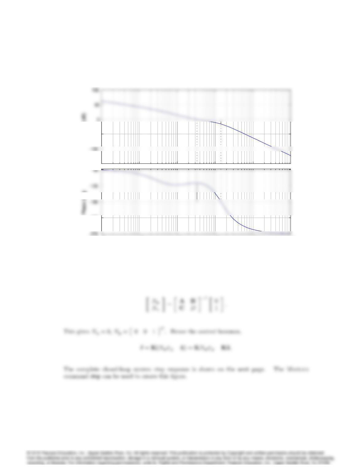
(e) The Bode plot of the closed-loop system is shown on the next page. The Matlab command
Bode or Margin can be used to create this figure. Note that when you find the Bode plot, the
7088 CHAPTER 7. STATE-SPACE DESIGN
–150
–50
Magnitude ( dB)
10
-3
10
-2
10
-1
10
0
10
1
10
2
–225
Bode D iagram
Gm = 15.8 dB (at 1.42 rad/sec) , Pm = 52.8 deg (at 0.334 rad/sec)
Frequency (rad/sec)
–150
–50
Magnitude ( dB)
10
-3
10
-2
10
-1
10
0
10
1
10
2
–225
Problem 7.55: Bode plot of closed-loop system for ship control.
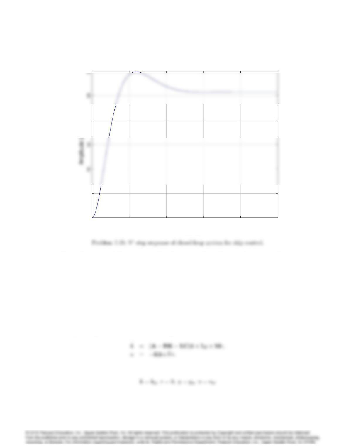
(f) Consider the determination of the feedforward gains Nxand Nuby,
7089
010 20 30 40 50
0
1
4
T i m e (se cs)
010 20 30 40 50
0
1
4
T i m e (se cs)
Problems and Solutions for Section 7.9: Introduction of the
Reference Input with the Estimator
56. NAs mentioned in footnote 11 in Section 7.9.2, a reasonable approach for selecting the feed-
forward gain in Eq. (7.202) is to choose
Nsuch that when rand yare both unchanging, the
DC gain from rto uis the negative of the DC gain from yto u: Derive a formula for
Nbased
on this selection rule. Show that if the plant is type 1, this choice is the same as that given by
Eq. (7.202).
Solution:
The system equations with the feedforward gains included are,
To find the DC gain from yto u, we let,
7090 CHAPTER 7. STATE-SPACE DESIGN
Then,
So that the DC gain from yto uis given by,
Similarly, to find the DC gain from rto u, we let,
Then,
So that the DC gain from rto uis given by,
From the footnote in the Servodesign section, we set the DC gain from rto uequal to the
negative of the DC gain from yto u,
We can show, in general, if
Nis chosen as the footnote implies, then the system DC gain is
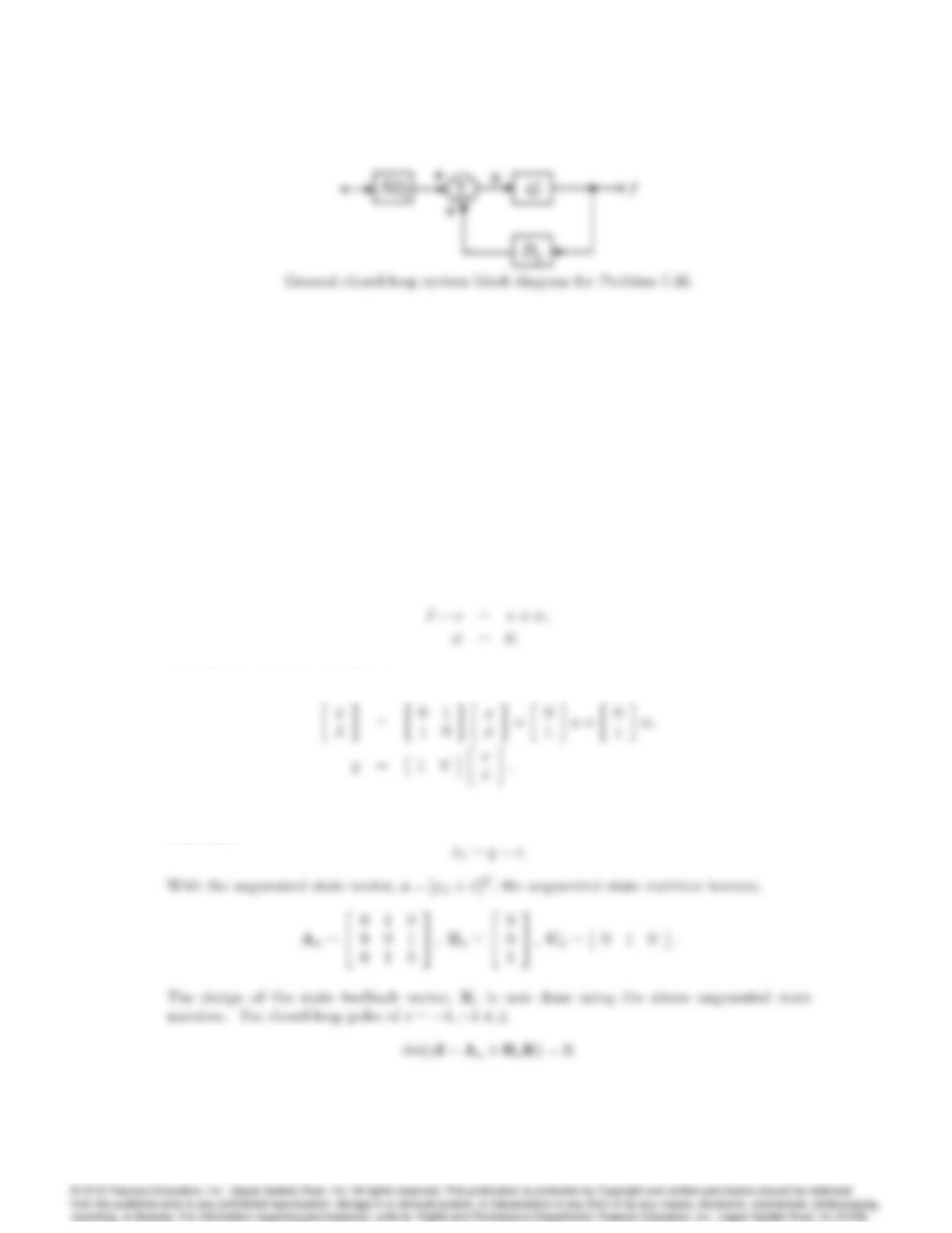
unity for a type I plant. Consider the general closed-loop system block diagram shown below.
7091
Problems and Solutions for Section 7.10: Integral Control
and Robust Tracking
57. Assume that the linearized and time-scaled equation of motion for the ball-bearing levitation
device is •xx=u+w. Here wis a constant bias due to the power amplifier. Introduce integral
error control, and select three control gains K= [ K1K2K3]so that the closed-loop poles
are at 1and 1jand the steady-state error to wand to a (step) position command will
be zero. Let y=xand the reference input r,yref be a constant. Draw a block diagram of
your design showing the locations of the feedback gains Ki. Assume that both _xand xcan
be measured. Plot the response of the closed-loop system to a step command input and the
response to a step change in the bias input. Verify that the system is type 1. Use Matlab
(Simulink) software to simulate the system responses.
Solution:
The equations of motion are given by,
A realization of these equations is,
In order to incorporate integral control, we augment the state vector with an integral state, xI,
such that,
7092 CHAPTER 7. STATE-SPACE DESIGN
when,
The closed-loop system is given by,
To show that the system is Type I, show that y= 0 for any constant win the steady-state, i.e.,
This immediately gives z2= 0 and y=z2= 0. Thus, in steady-state y= 0 for any constant
0 2 4 6 8 10 12 14 16
0.6
1.4
T i m e (se cs)
Amplitude
0 2 4 6 8 10 12 14 16
0.6
1.4
T i m e (se cs)
Amplitude
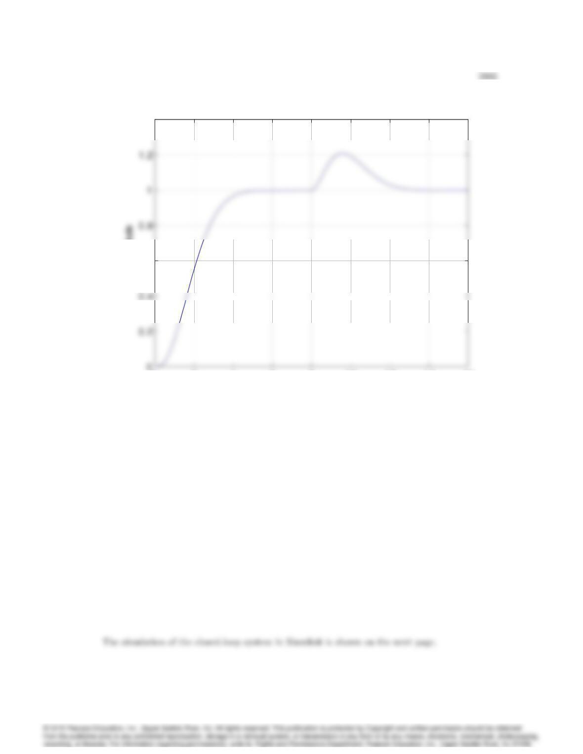
Problem 7.57: Response of closed-loop system to a unit step input at t= 0 and step
disturbance at t= 8.
x2 x1
St ep
Integrator3
-2
Gain1
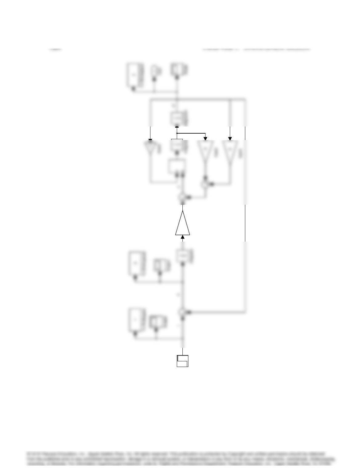
Simulink simulation for Problem 7.57.
58. Consider a system with state matrices,
A=2 1
03;B=1
1;C= [ 1 3 ]:
a) Use feedback of the form u(t) = Kx(t) +
Nr(t), where
Nis a nonzero scalar, to move the
poles to 33j.
b) Choose
Nso that if ris a constant, the system has zero steady-state error; that is y(1) = r.
c) Show that if Achanges to A+A, where Ais an arbitrary 22matrix, then your choice of
Nin part (b) will no longer make y(1) = r. Therefore, the system is not robust under changes
to the system parameters in A.
d) The system steady-state error performance can be made robust by augmenting the system
with an integrator and using unity feedback; that is, by setting _xI=ry, where xIis the state
of the integrator. To see this, first use state feedback of the form u=Kx K1xIso that the
poles of the augmented system are at 3;2jp3.
e) Show that the resulting system will yield y(1) = rno matter how the matrices Aand B
are changed, as long as the closed-loop system remains stable.
f) For part (d), use Matlab (Simulink) software to plot the time response of the system to a
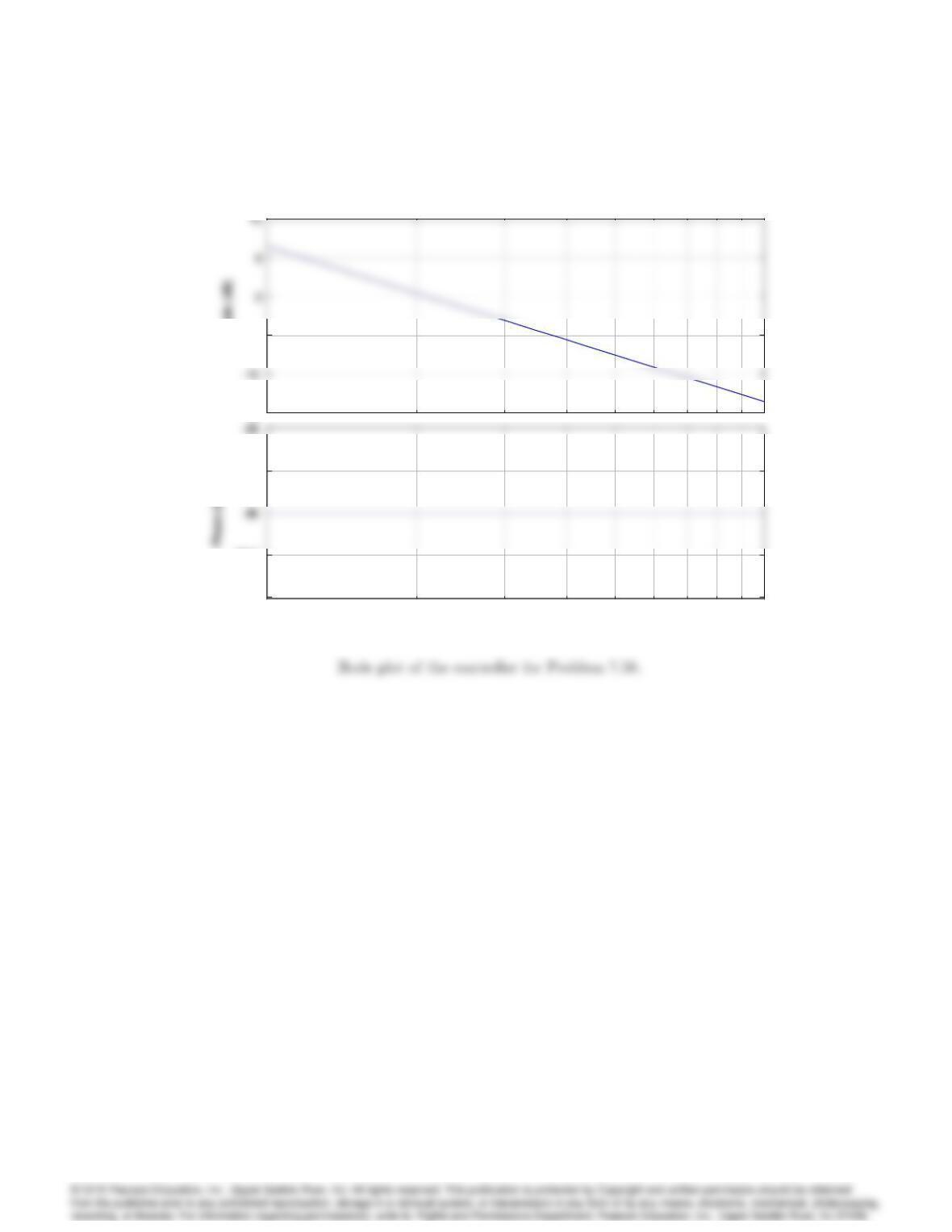
constant input. Draw Bode plots of the controller as well as the sensitivity function (S) and
the complementary sensitivity function (T).
Solution:
(a) Using feedback of the form, u=Kx +Nr; we have,
(b) We can find the desired value for Nby setting the DC gain from rto yequal to unity. The
closed-loop system equations are,
and the DC gain is simply,
(c) Change Ato (A+A), and let the value of Nthat keeps the tracking error at zero be N0.
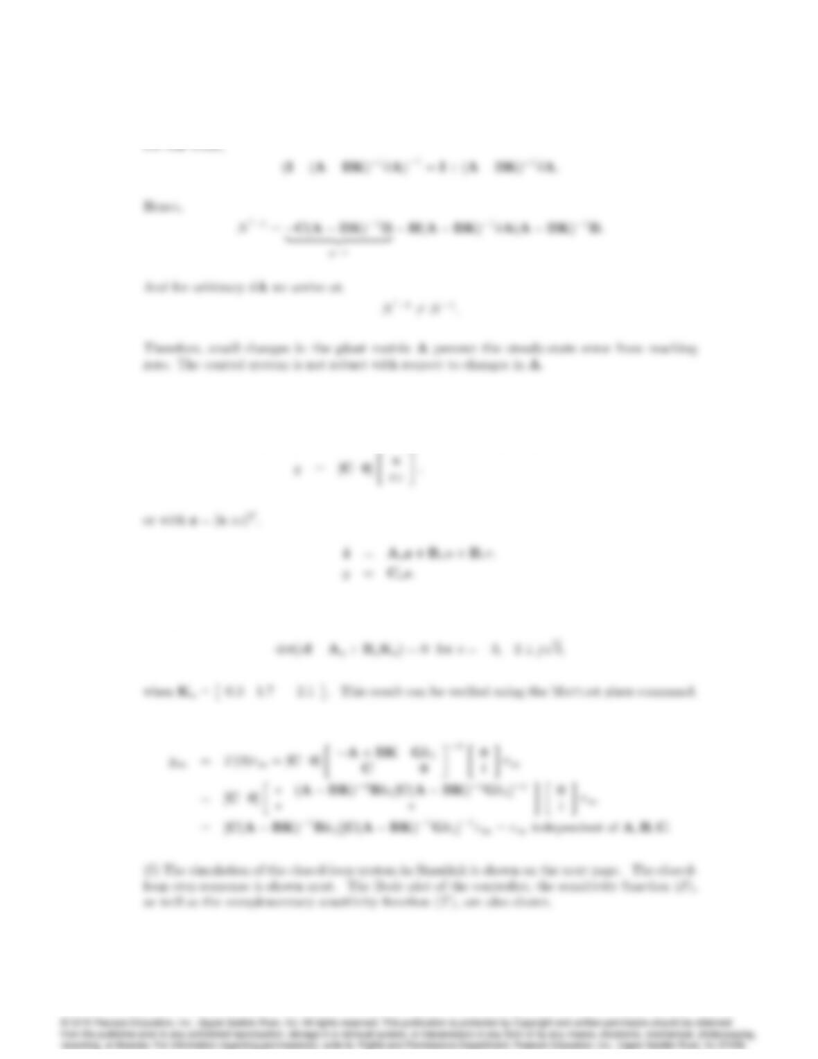
7096 CHAPTER 7. STATE-SPACE DESIGN
(d) Augmenting the system equations with an integrator state, xI, the state equation become,
_x
_xI=A 0
C0 x
xI+B
0u+0
1r;
Using feedback of the form u=Kx kIxI=Kaz, we have,
(e) We can show that the closed-loop DC gain from rto yis independent of A,
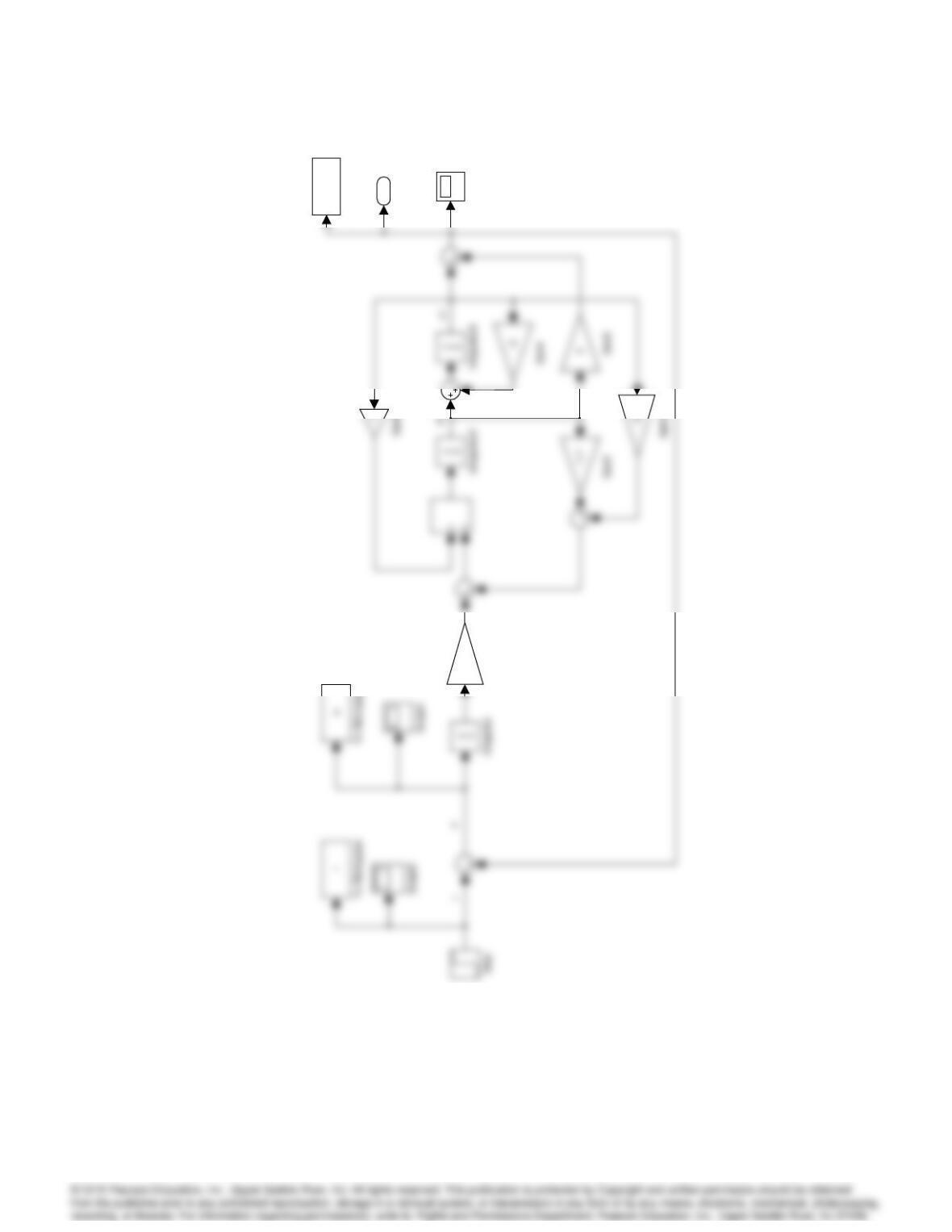
7097
e
1
Out1
y
T o Workspace1
Scope
–2.1
Gain1
Simulink simulation for Problem 7.58.
7098 CHAPTER 7. STATE-SPACE DESIGN
00.5 11.5 22.5 33.5 44.5 5
0.4
0.8
1.4
Time (sec)
Amplitude
00.5 11.5 22.5 33.5 44.5 5
0.4
0.8
1.4
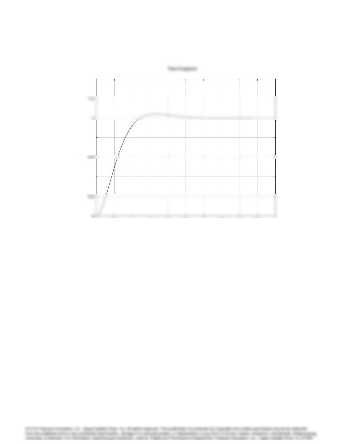
Closed-loop step response for Problem 7.58.
7099
–15
-5
Magnitude ( dB)
10
0
10
1
–91
–90.5
–89.5
Bode D iagram
Frequency (rad/sec)
–15
-5
Magnitude ( dB)
10
0
10
1
–91
–90.5
–89.5