7020 CHAPTER 7. STATE-SPACE DESIGN
(b)
Y(s)
U(s)=G(s) = 3s+ 4
s2+ 2s+ 2:
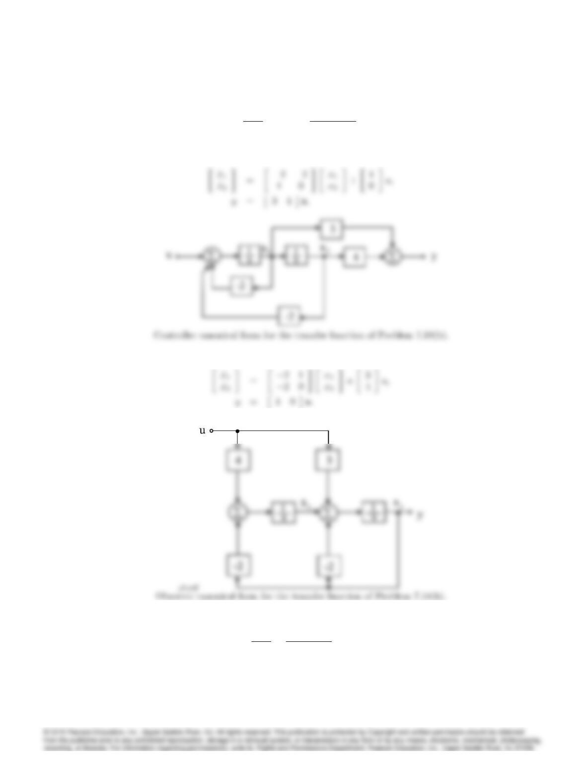
This transfer function can be realized in Controller canonical form as shown below. From the
figure, we have,
The block diagram for observer canonical form is shown below. From the figure, we have:
19. Consider the transfer function,
G(s) = Y(s)
U(s)=s+ 6
s2+ 5s+ 6:(7:283)
7021
a) By rewriting Eq. (7.283) in the form,
G(s) = 1
s+ 3 s+ 6
s+ 2;
find a series realization of G(s)as a cascade of two first-order systems.
b) Using a partial-fraction expansion of G(s), find a parallel realization of G(s).
c) Realize G(s)in control canonical form.
Solution:
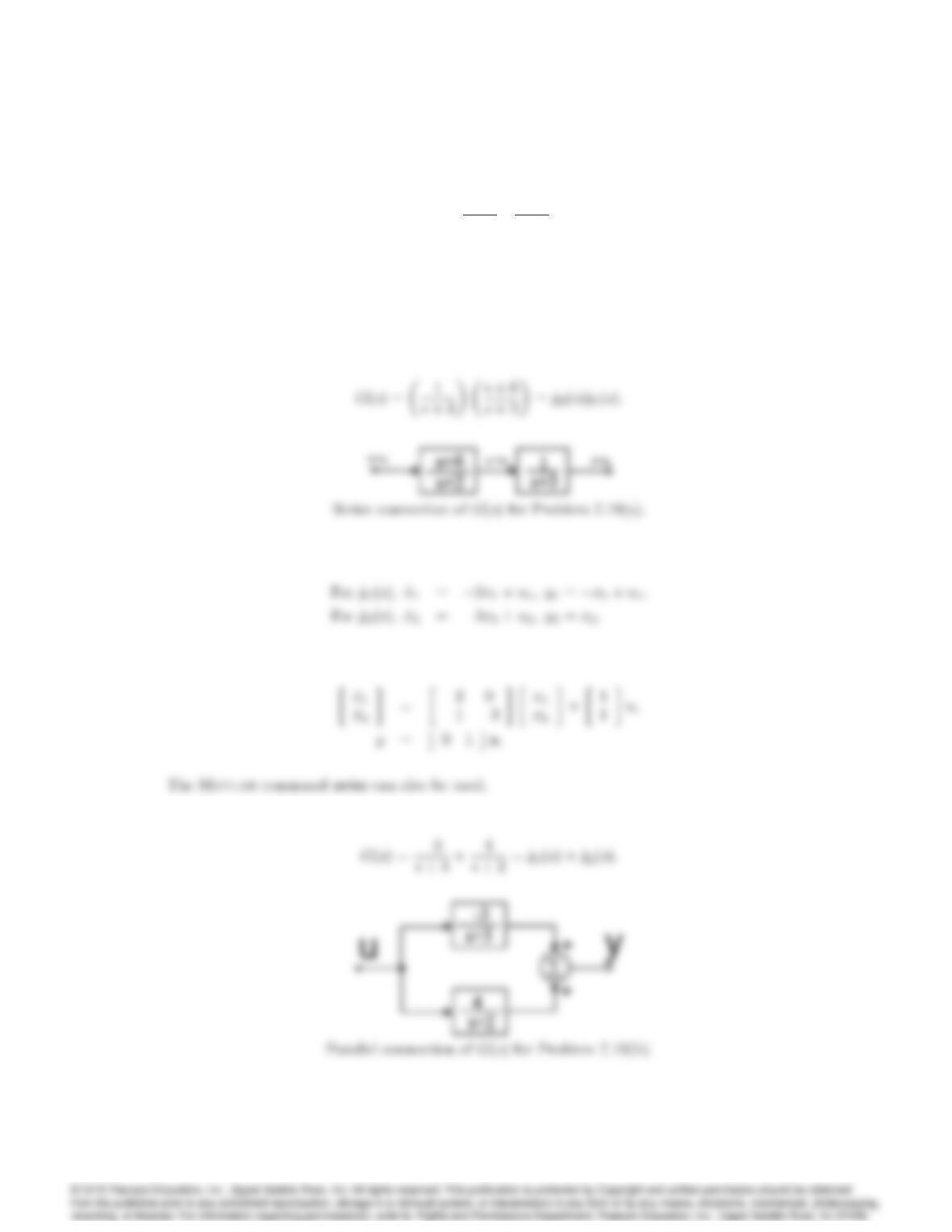
(a) The series realization shown below is given by:
The series interconnections result in u=u1; y =y2; u2=y1. Therefore,
(b) The parallel realization, shown below, is given by:
7022 CHAPTER 7. STATE-SPACE DESIGN
The interconnections are u1=u2=u; y =y1+y2. Therefore,
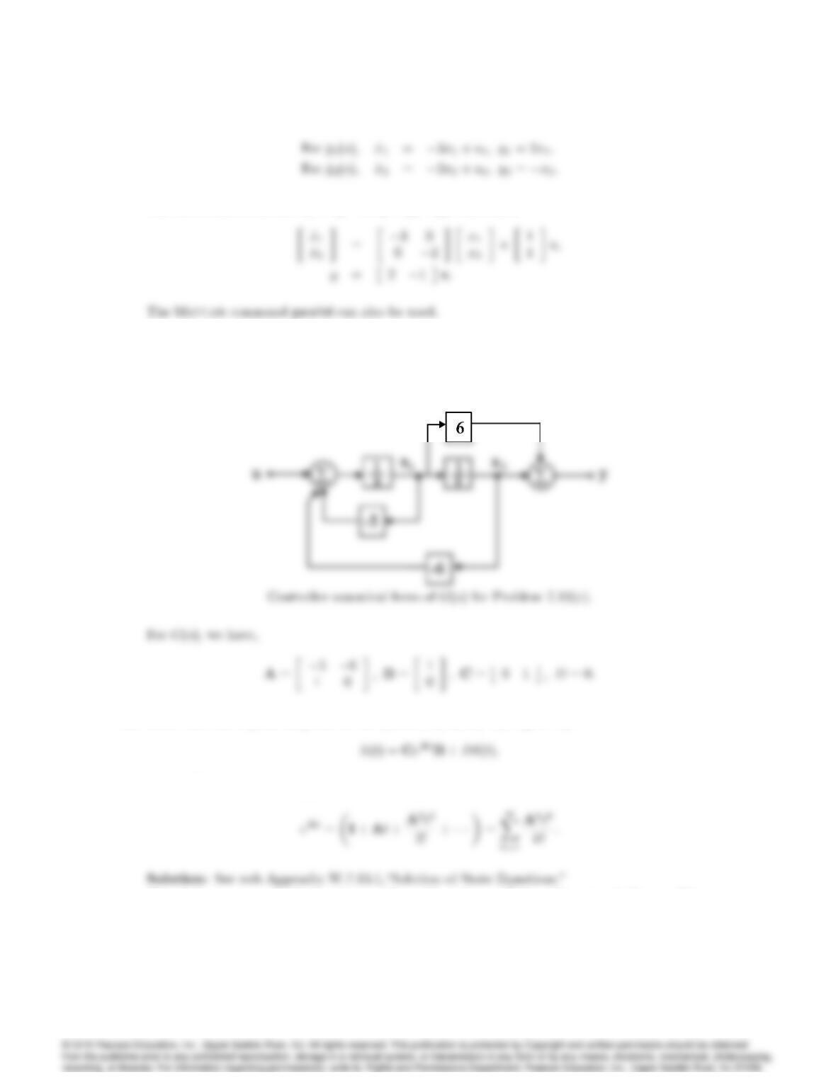
(c) Control canonical form, shown in Fig. 7.17, is realized by simply picking off the appropriate
coefficients of the original (strictly proper) transfer function. If the original transfer function is
not strictly proper, then it should be reduced to a feedthrough term (D) plus a strictly proper
transfer function term.
20. Show that the impulse response of the system (A,B,C,D) is given by
where eAtis the matrix exponential defined by
Problems and Solutions for Section 7.5: Control-Law De–
sign for Full-State Feedback
21. Consider the plant described by,
_
x=0 1
74x+1
2u;
y= [ 1 3 ]x:
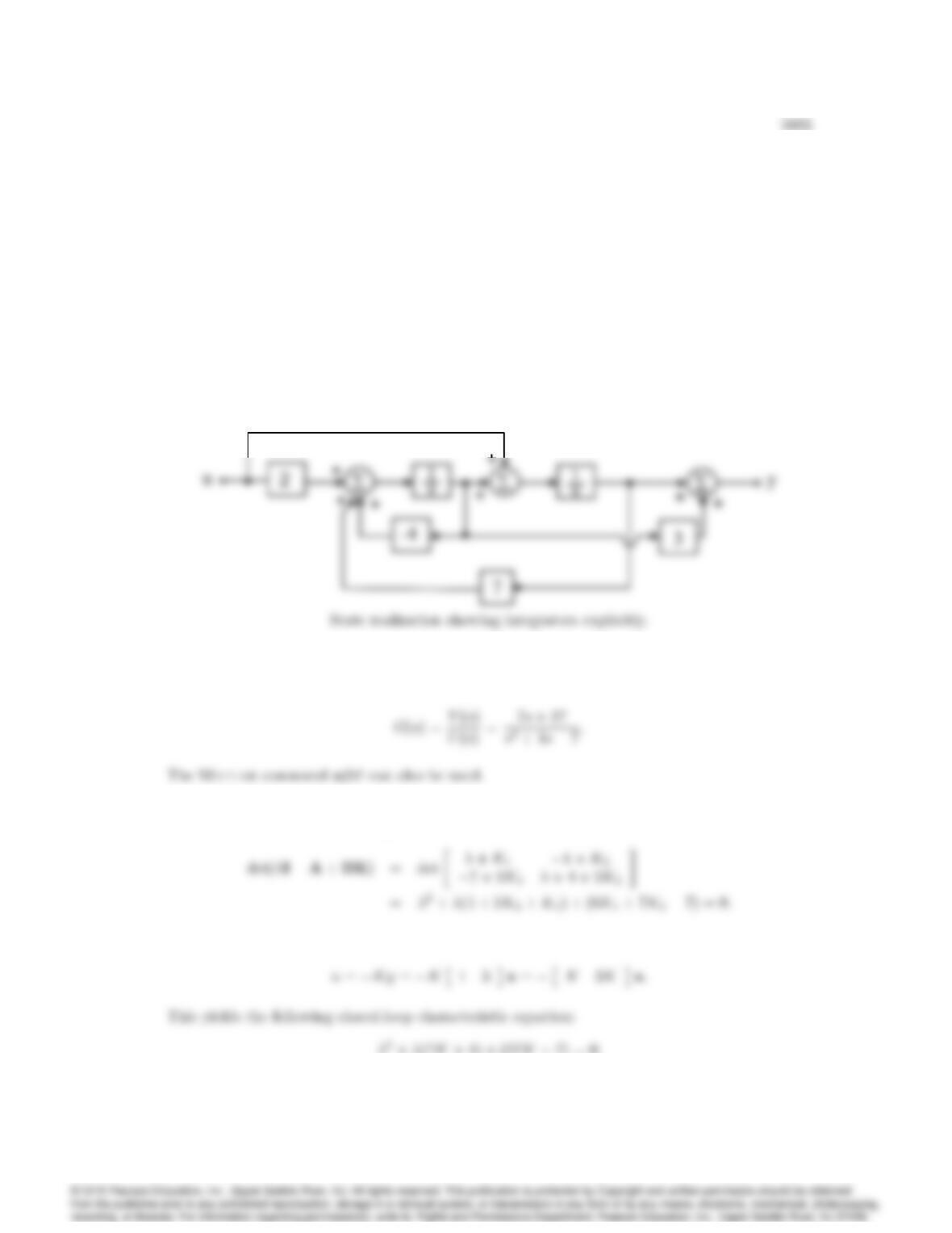
a) Draw a block diagram for the plant with one integrator for each state variable.
b) Find the transfer function using matrix algebra.
c) Find the closed-loop characteristic equation if the feedback is
(1) u=[K1K2]x; (2) u=Ky.
Solution:
(a) See figure.
(b) Using the formula G(s) = C(sIA)1B, we obtain,
(c)
(i) State feedback, u=[K1K2]x.
(ii) Output feedback,
2+(7K+ 4) + (27K7) = 0:
22. For the system,
_
x=0 1
65x+0
1u;
y=1 0 x;
design a state feedback controller that satisfies the following specifications:
Closed-loop poles have a damping coefficient = 0:707.
Step-response peak time is under 3.14 sec.
Verify your design with Matlab.
Solution:
Using state feedback u=Kx, we get,
Hence the closed-loop characteristic equation is,
7025
0 1 2 3 4 5 6
0.4
0.6
Step Response
Time (sec)
Amplitude
0 1 2 3 4 5 6
0.4
0.6
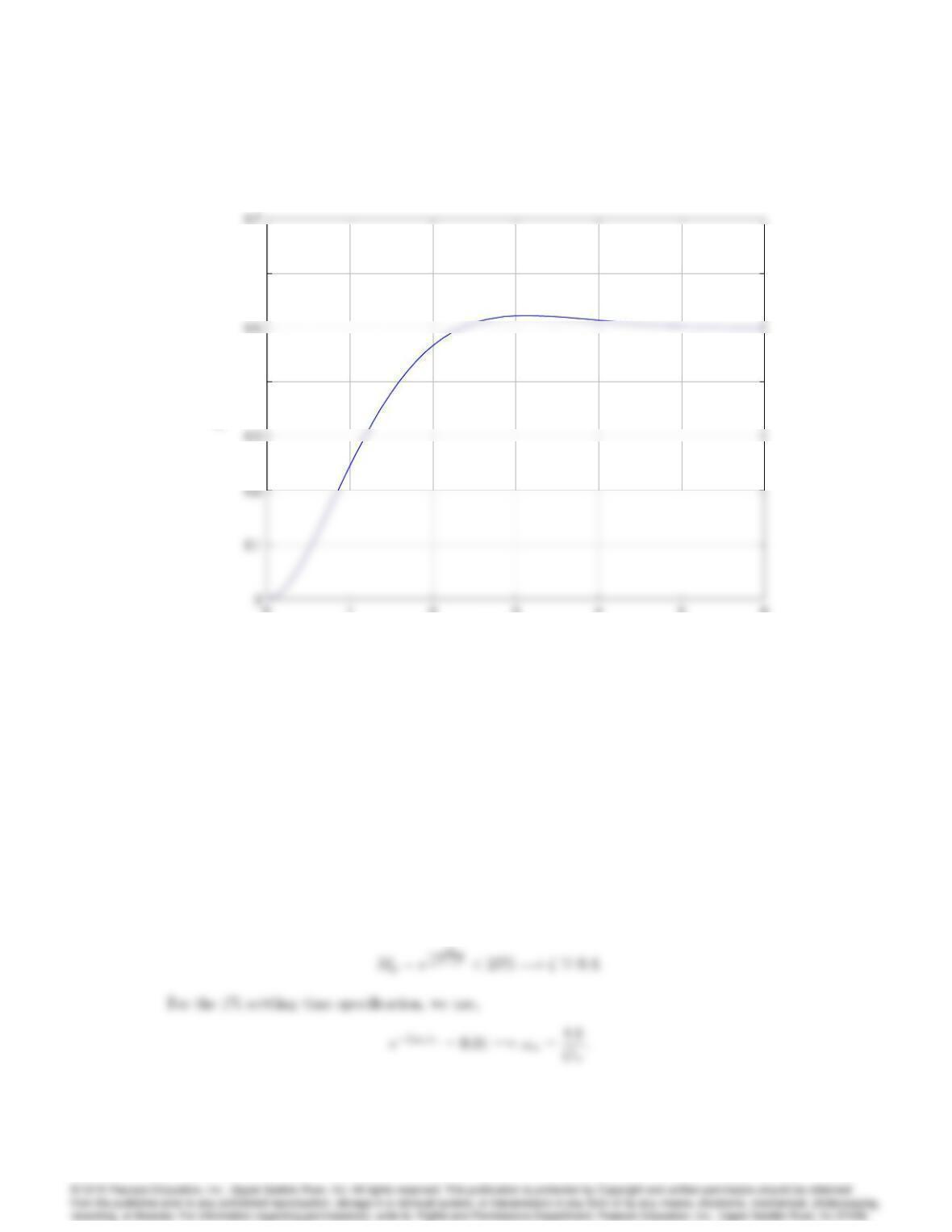
Step response for Problem 7.22.
23. a) Design a state feedback controller for the following system so that the closed-loop step response
has an overshoot of less than 25% and a 1% settling time under 0.115 sec.:
_
x=0 1
010 x+0
1u;
y=1 0 x:
b) Use the step command in Matlab to verify that your design meets the specifications. If it
does not, modify your feedback gains accordingly.
Solution:
(a) For the overshoot specification,
7026 CHAPTER 7. STATE-SPACE DESIGN
(b) This can be implemented in Matlab with the following code:
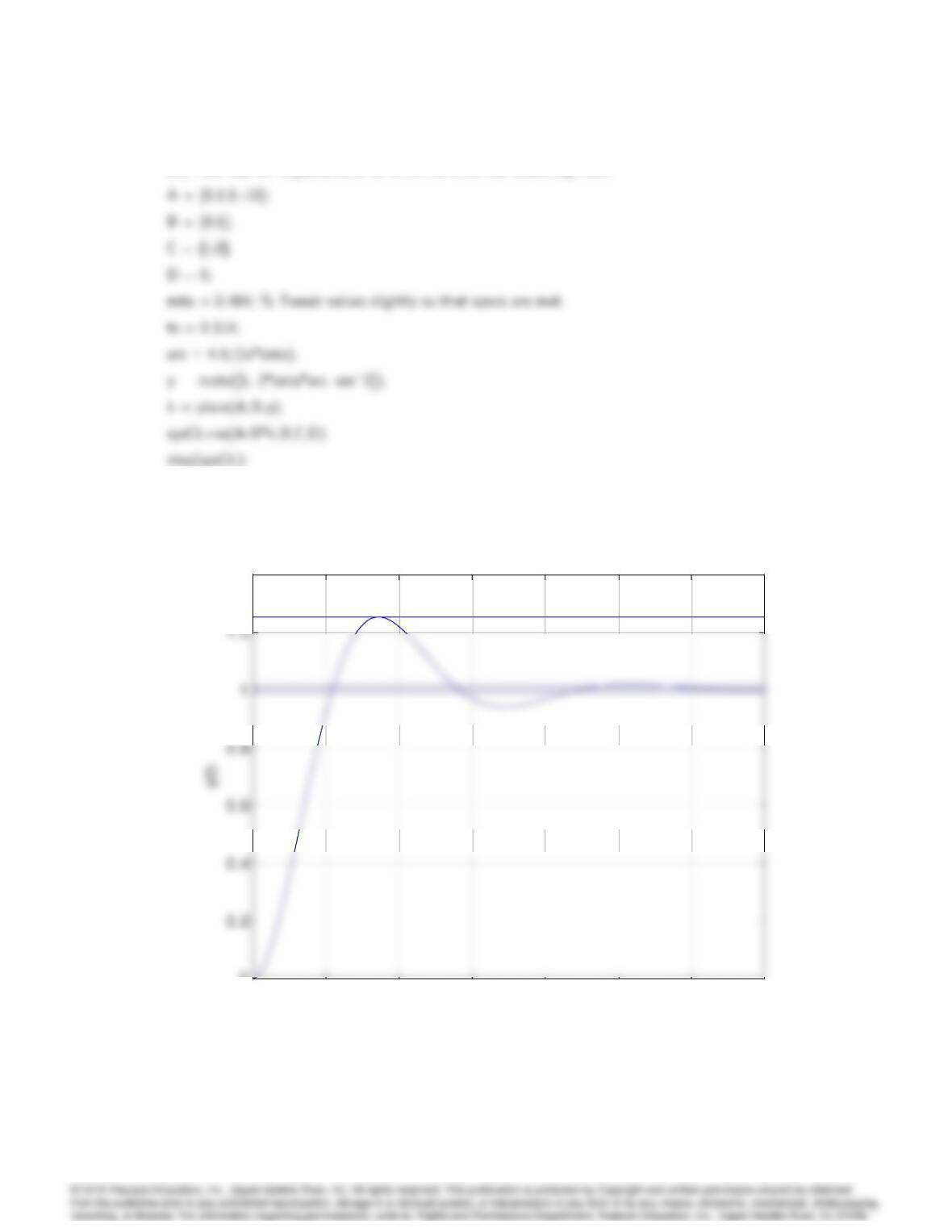
The step response is shown next.
00.02 0.04 0.06 0.08 0.1 0.12 0.14
0
1.4 x 10
-4 Control design with overshoot and settling time specs
Time (sec)
00.02 0.04 0.06 0.08 0.1 0.12 0.14
0
1.4 x 10
-4 Control design with overshoot and settling time specs
Time (sec)
Step response for Problem 7.23.
24. Consider the system,
_
x=2
4
122
01 1
1 0 1
3
5x+2
4
2
0
1
3
5u;
y=100x:
a) Design a state feedback controller for the system so that the closed-loop step response has an
overshoot of less than 5% and a 1% settling time under 4.6 sec.
b) Use the step command in Matlab to verify that your design meets the specifications. If it
does not, modify your feedback gains accordingly.
Solution:
(a) There are many different approaches to designing the control law. We will attack the problem
The open-loop poles are at 1:45 and 0:77 j1:47 and the open-loop zeros are at 1:37 and
function [k,p]=srl(A,B,C)
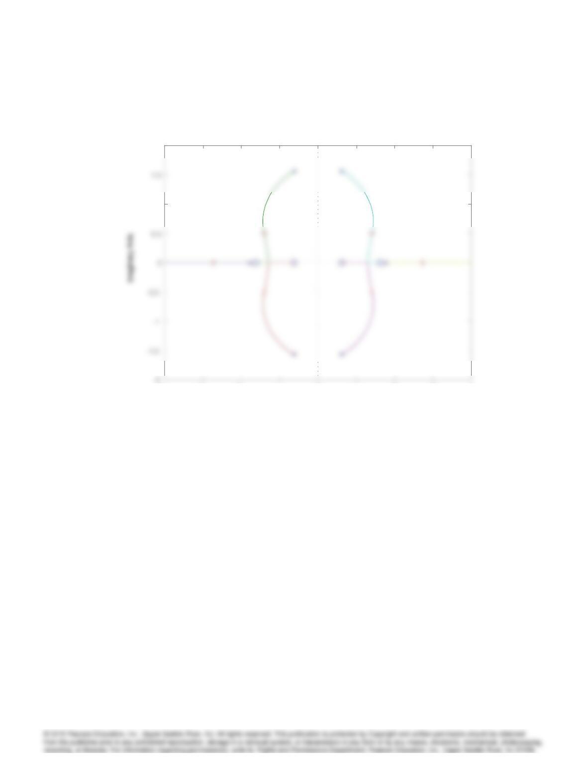
Note that crosses indicate where the closed-loop pole locations have been selected, which roughly
7028 CHAPTER 7. STATE-SPACE DESIGN
-4 -3 -2 -1 0 1 2 3 4
1
2
Root Locus
Real Axis
Symmetric root locus for Problem 7.24.
7029
00.5 11.5 22.5 33.5 44.5
-1
0.2
0.4
0.8
1
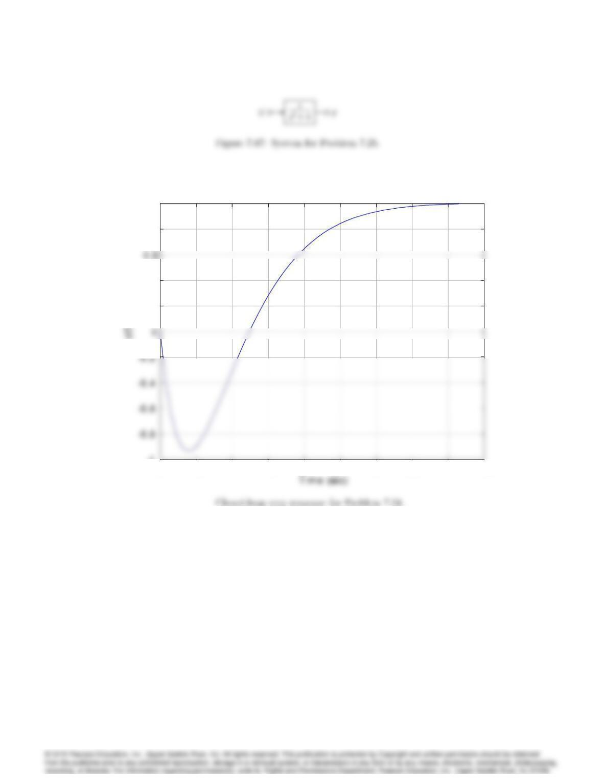
Control design with overshoot and settling time specs
00.5 11.5 22.5 33.5 44.5
-1
0.2
0.4
0.8
1
Control design with overshoot and settling time specs
25. Consider the system in Fig. 7.87.
a) Write a set of equations that describes this system in the control canonical form as _
x=
Ax +Buand y=Cx.
b) Design a control law of the form,
u=[K1K2]x1
x2;
which will place the closed-loop poles at s=22j:
Solution:
(a) Let’s write this system in the control canonical form,
7030 CHAPTER 7. STATE-SPACE DESIGN
26. Output Controllability: In many situations a control engineer may be interested in controlling
the output yrather than the state x. A system is said to be output controllable if at any time
you are able to transfer the output from zero to any desired output yin a finite time using an
appropriate control signal u. Derive necessary and sufficient conditions for a continuous system
(A,B,C) to be output controllable. Are output and state controllability related? If so, how?
Solution:
Because we are considering linear systems, if you can take the state from some initial state to
then
7031
Therefore, a system is output controllable if and only if,
27. Consider the system,
_x =2
6
6
4
0 4 0 0
14 0 0
5 7 1 15
0 0 3 3
3
7
7
5x+2
6
6
4
0
0
1
0
3
7
7
5u:
a) Find the eigenvalues of this system. (Hint: Note the block-triangular structure.)
b) Find the controllable and uncontrollable modes of this system.
c) For each of the uncontrollable modes, find a vector vsuch that,
vTB= 0;vTA=vT:
d) Show that there are an infinite number of feedback gains Kthat will relocate the modes of
the system to 5,3,2, and 2.
e) Find the unique matrix Kthat achieves these pole locations and prevents initial conditions
on the uncontrollable part of the system from ever affecting the controllable part.
Solution:
(a) Because the system is block lower triangular, we can determine the eigenvalues of the system
by taking the union of the eigenvalues of each of the blocks along the main (block)diagonal.
(b) To find the controllable or uncontrollable modes of the system, we follow method learned
in Problem 7.28. Specifically, we find an orthogonal similarity transformation which transforms
7032 CHAPTER 7. STATE-SPACE DESIGN
Matlab function ctrbf will give a similar result, although the order of the state variables may
be switched.
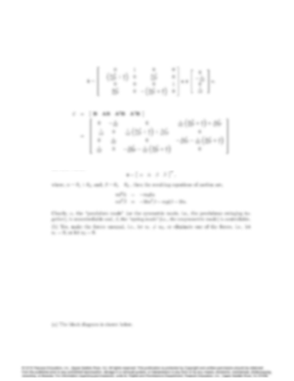
28. Two pendulums, coupled by a spring, are to be controlled by two equal and opposite forces u,
which are applied to the pendulum bobs as shown in Fig. 7.88. The equations of motion are
ml2•
1=ka2(12)mgl1lu;
ml2•
2=ka2(21)mgl2+lu:
a) Show that the system is uncontrollable. Can you associate a physical meaning with the
controllable and uncontrollable modes?
b) Is there any way that the system can be made controllable?
7033
Solution:
(a) Using the state vector x= [1_
12_
2]T;
The controllability matrix is determined as,
Then (A,B) is uncontrollable since det(C)=0. If we re-write the state equations in terms of
the state vector,
29. The state-space model for a certain application has been given to us with the following state
description matrices:
A=
2
6
6
6
6
4
0:174 0 0 0 0
0:157 0:645 0 0 0
0 1 0 0 0
0 0 1 0 0
0 0 0 1 0
3
7
7
7
7
5
;B=
2
6
6
6
6
4
0:207
0:005
0
0
0
3
7
7
7
7
5
;C= [ 10000]:
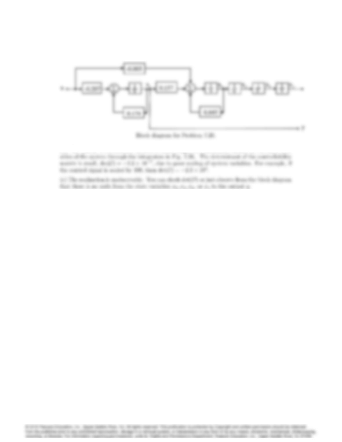
a) Draw a block diagram of the realization with an integrator for each state variable.
b) A student has computed det C= 2:3107and claims that the system is uncontrollable. Is
the student right or wrong? Why?
c) Is the realization observable?
Solution:
7034 CHAPTER 7. STATE-SPACE DESIGN
(b) The system is controllable because a control signal u(command) reaches all the state vari-
30. Staircase Algorithm (Van Dooren et al., 1978): Any realization (A,B,C) can be transformed
by an orthogonal similarity transformation to (
A,
B,
C), where
Ais an upper Hessenberg
matrix (having one nonzero diagonal above the main diagonal):
A=TTAT =
2
6
6
6
6
4
100
...0
...n1
3
7
7
7
7
5
;
B=TTB=
2
6
6
6
6
6
4
0
0
.
.
.
0
g1
3
7
7
7
7
7
5
;
where g16= 0, and,
C=CT = [c1c2 cn];T1=TT:
Orthogonal transformations correspond to a rotation of the vectors (represented by the matrix
columns) being transformed with no change in length.
a) Prove that if i= 0 and i+1; : : : ; n16= 0 for some i, then the controllable and uncontrol-
lable modes of the system can be identified after this transformation has been done.
b) How would you use this technique to identify the observable and unobservable modes of (A,
B,C)?
c) What advantage does this approach for determining the controllable and uncontrollable modes
have over transforming the system to any other form?
d) How can we use this approach to determine a basis for the controllable and uncontrollable
subspaces, as in Problem 7.44?
This algorithm can be used to design a numerically stable algorithm for pole placement [see
Minimis and Paige (1982)]. The name of the algorithm comes from the multi-input version in
which the iare the blocks that make
Aresemble a staircase.
Solution:
7035
(a) If i= 0,
2
10 0 0 0 0 0
3
2
0
3
This suggests naturally splitting up the state vector into two parts x= [x1x2]Twhere x1and
x2are vectors of the appropriate size (depending upon which i= 0). Then recognize that the
equations are,
Problems and Solutions for Section 7.6: Selection of Pole
Locations for Good Design
31. The normalized equations of motion for an inverted pendulum at angle on a cart are,
•
=+u; •x= u;
where xis the cart position, and the control input uis a force acting on the cart.
a) With the state defined as x= [; _
; x; _x]T, find the feedback gain Kthat places the closed-
loop poles at s=1;1;11j.
For parts (b) through (d), assume that = 0:5.
b) Use the symmetric root locus to select poles with a bandwidth as close as possible to those of
7036 CHAPTER 7. STATE-SPACE DESIGN
part (a), and find the control law that will place the closed-loop poles at the points you selected.
c) Compare the responses of the closed-loop systems in parts (a) and (b) to an initial condition
of = 10. You may wish to use the initial command in Matlab.
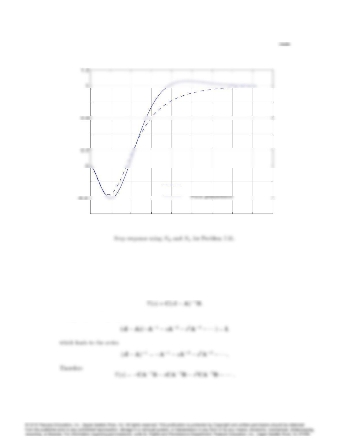
d) Compute Nxand Nufor zero steady-state error to a constant command input on the cart
position, and compare the step responses of each of the two closed-loop systems.
Solution:
(a) The state space equations of motion are,
2
_
3
3
3
3
From the above state equations,
Comparing coefficients yields:
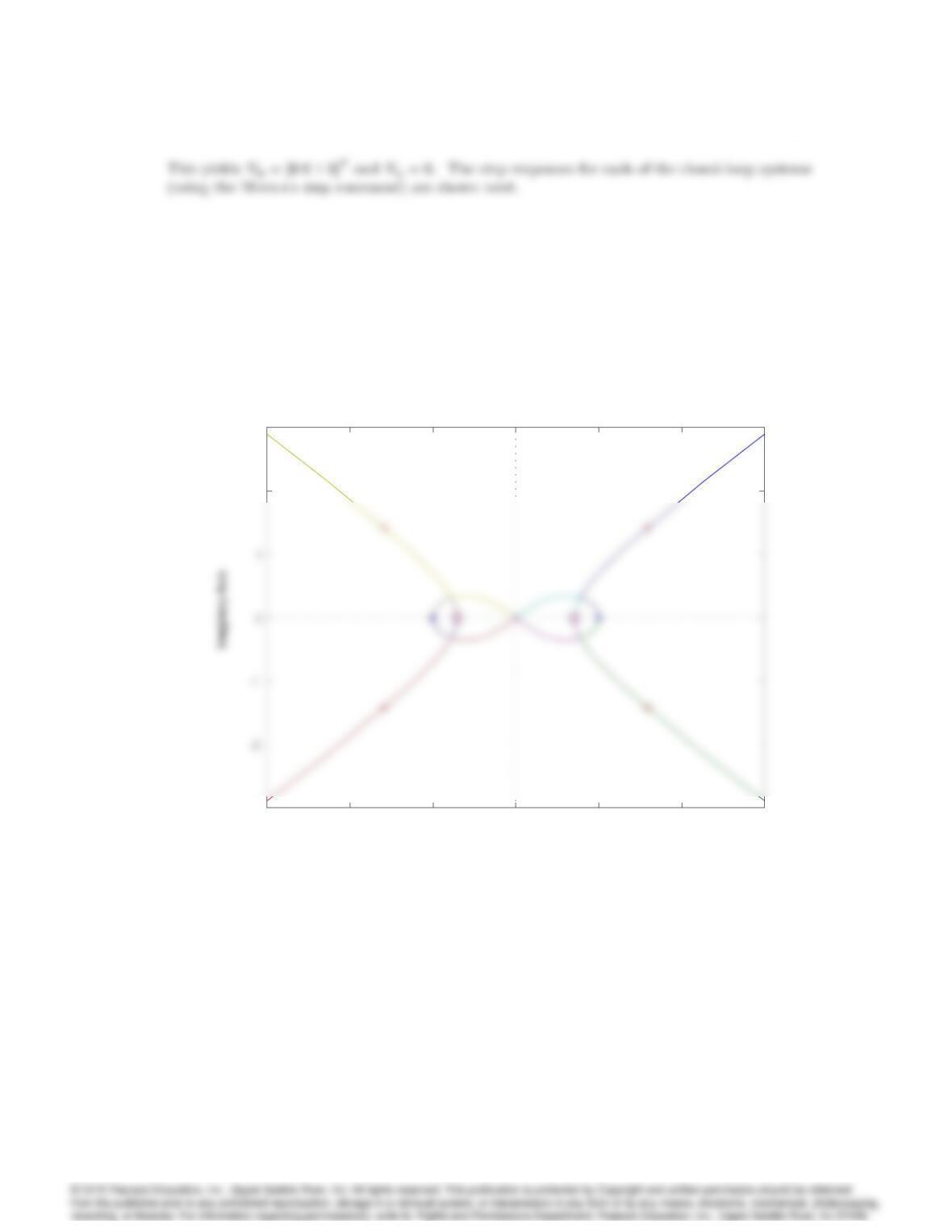
(b) The symmetric root locus is shown below, where we have chosen C=0010. The
following Matlab commands can be used to generate the symmetric root locus,
% Symmetric root locus
7037
-3 -2 -1 0 1 2 3
-3
2
3
Root Locus
Real Axis
Symmetric root locus for Problem for Problem 7.31.
7038 CHAPTER 7. STATE-SPACE DESIGN
0 1 2 3 4 5 6 7 8 9
-5
5
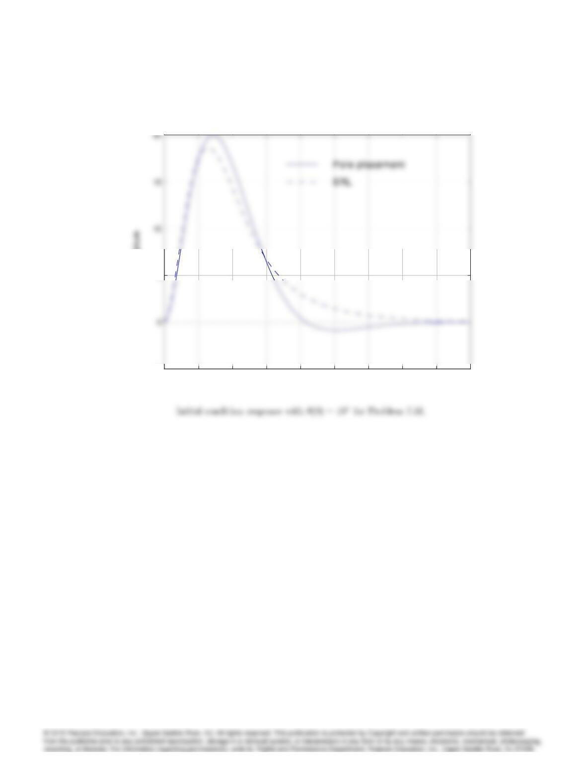
Response to Initial C onditions
Time (sec)
Amplitude
0 1 2 3 4 5 6 7 8 9
-5
5
0 1 2 3 4 5 6 7 8 9
–0.6
–0.2
0.4
0.8
SRL
0 1 2 3 4 5 6 7 8 9
–0.6
–0.2
0.4
0.8
SRL
32. An asymptotically stable type I system with input rand output yis described by the closed-loop
system matrices (A,B,C,D= 0). Suppose the input is given by the ramp r=at, for t > 0.
Show that the velocity error coefficient, Kv, for this system is given by
Kv=CA2B1:
Solution: The closed-loop transfer function is
Asymptotic stability implies that Ais invertible. We can write that