7060 CHAPTER 7. STATE-SPACE DESIGN
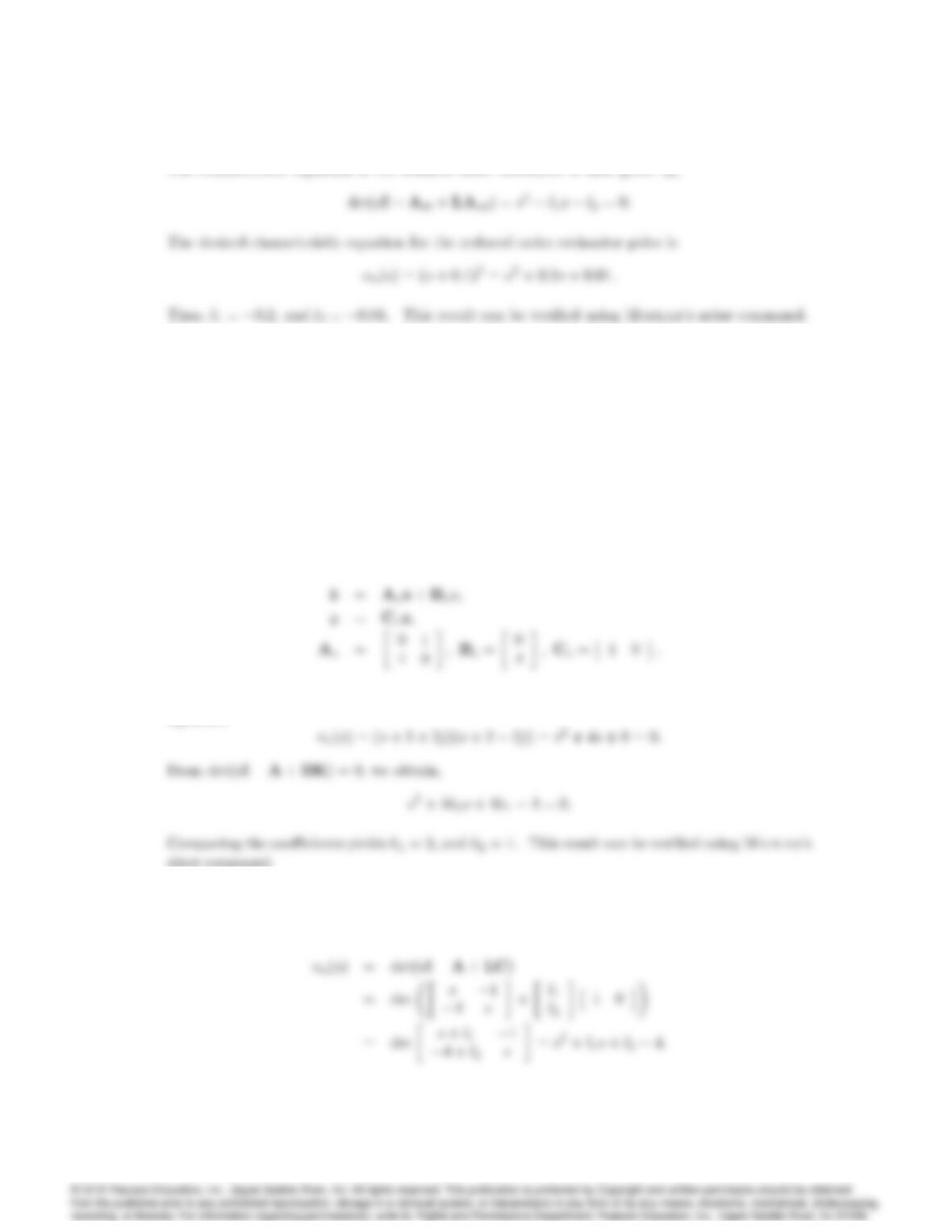
The characteristic equation of the reduced order estimator is then given by,
Problems and Solutions for Section 7.8: Compensator De–
sign: Combined Control Law and Estimator
48. A certain process has the transfer function G(s) = 4=(s24).
a) Find A,B, and Cfor this system in observer canonical form.
b) If u=Kx, compute Kso that the closed-loop control poles are located at s=22j.
c) Compute Lso that the estimator-error poles are located at s=10 10j.
d) Give the transfer function of the resulting controller (for example, using Eq. (7.177)).
e) What are the gain and phase margins of the controller and the given open-loop system?
Solution:
(a) From the transfer function, we can read off the elements that will give observer canonical
form,
(b) With u=[k1k2][x1x2]T, we want to achieve the following closed-loop characteristic
equation:
place command.
(c) The estimator roots are determined by the equation e(s) = 0. We want to find l1and l2
such that,
e(s) = (s+ 10 + 10j)(s+ 10 10j) = s2+ 20s+ 200:
7061
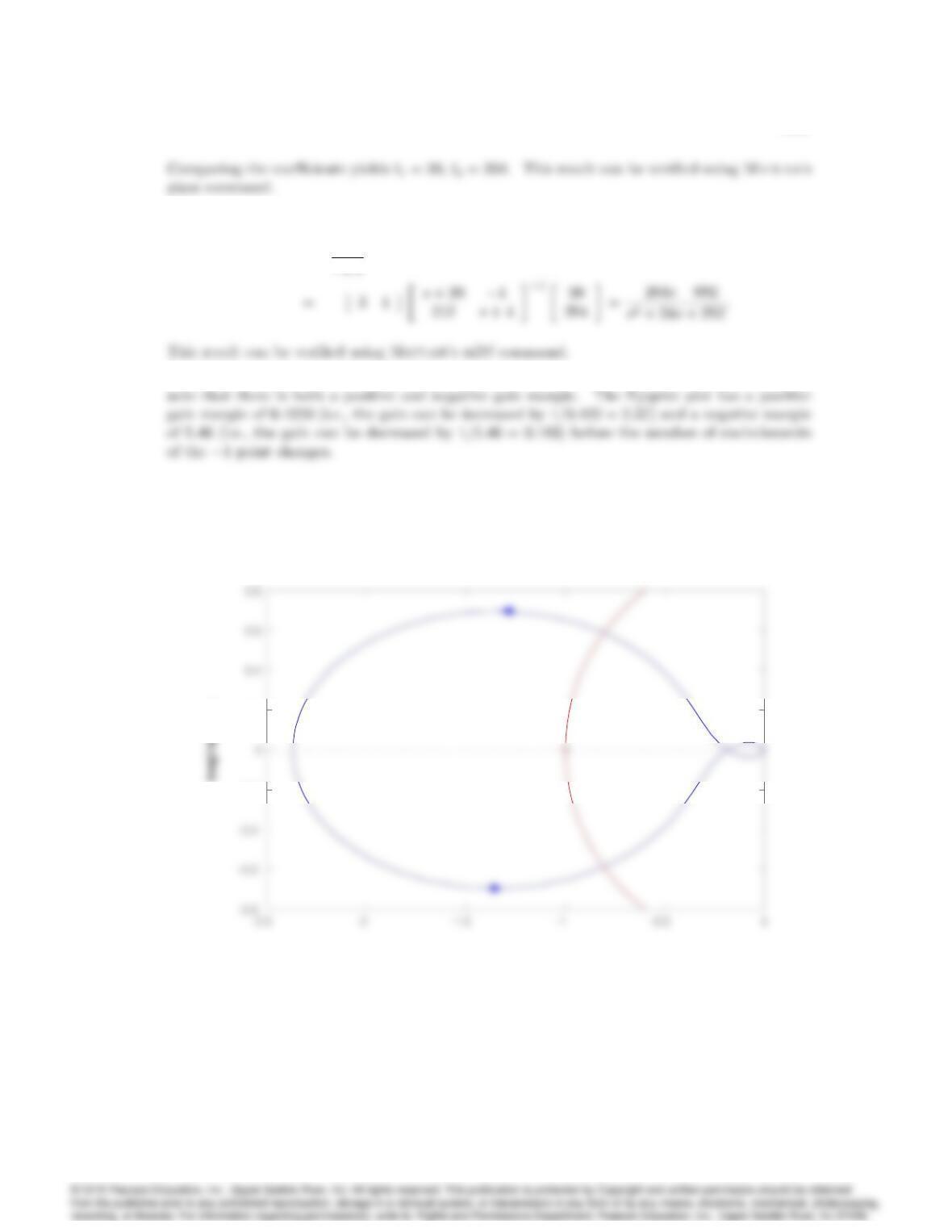
(d) The transfer function of the resulting compensator is,
Dc(s) = U(s)
Y(s)=K(sIA+BK +LC)1L;
(e) The next figure shows the Nyquist plot generated by Matlab (using the nyquist command),
–0.2
0.2
Nyquist Diag r am
Real Axis
Nyquist plot for Problem 7.48.
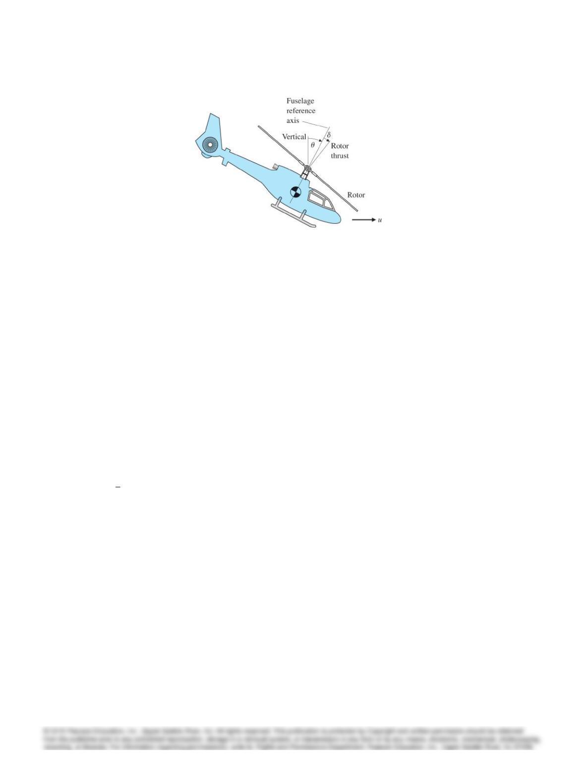
49. The linearized longitudinal motion of a helicopter near hover (Fig. 7.97) can be modeled by the
7062 CHAPTER 7. STATE-SPACE DESIGN
Figure 7.97: Helicopter for Problem 7.49.
normalized third-order system,
2
4
_q
_
_u3
5=2
40:4 0 0:01
1 0 0
1:4 9:80:02 3
52
4
q
u3
5+2
4
6:3
0
9:83
5;
where,
q= pitch rate;
= pitch angle of fuselage;
u= horizontal velocity (standard aircraft notation);
= rotor tilt angle (control variable):
Suppose our sensor measures the horizontal velocity uas the output; that is, y=u.
a) Find the open-loop pole locations.
b) Is the system controllable?
c) Find the feedback gain that places the poles of the system at s=11jand s=2.
d) Design a full-order estimator for the system, and place the estimator poles at 8and 4
4p3j.
e) Design a reduced-order estimator with both poles at 4. What are the advantages and
disadvantages of the reduced-order estimator compared with the full-order case?
f) Compute the compensator transfer function using the control gain and the full-order estimator
designed in part (d), and plot its frequency response using Matlab. Draw a Bode plot for the
closed-loop design, and indicate the corresponding gain and phase margins.
g) Repeat part (f) with the reduced-order estimator.
h) Draw the symmetrical root locus (SRL) and select roots for a control law that will give a
control bandwidth matching the design of part (c), and select roots for a full-order estimator
that will result in an estimator error bandwidth comparable to the design of part (d). Draw
the corresponding Bode plot and compare the pole placement and SRL designs with respect to
bandwidth, stability margins, step response, and control effort for a unit-step rotor-angle input.
Use Matlab for the computations.
Solution:
7063
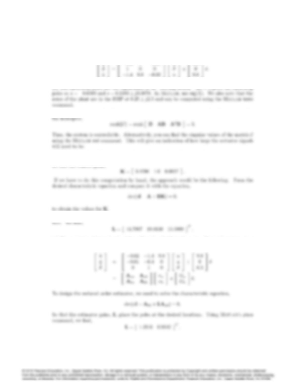
Again, the equations of motion for the helicopter are,
2
_q
q
6:3
(b) To determine controllability, we want to look at the rank of the controllability matrix. For
(c) When the order of the system gets larger than two, it is often convenient to let the computer
do the necessary calculations. Using Matlab’s place command and the specified pole locations,
(d) Using the duality principle, we find the estimator gains using Matlab’s place command as
(e) The notation of this solution follows Equation 7.139 in the text. Reordering the system
matrix, we have,
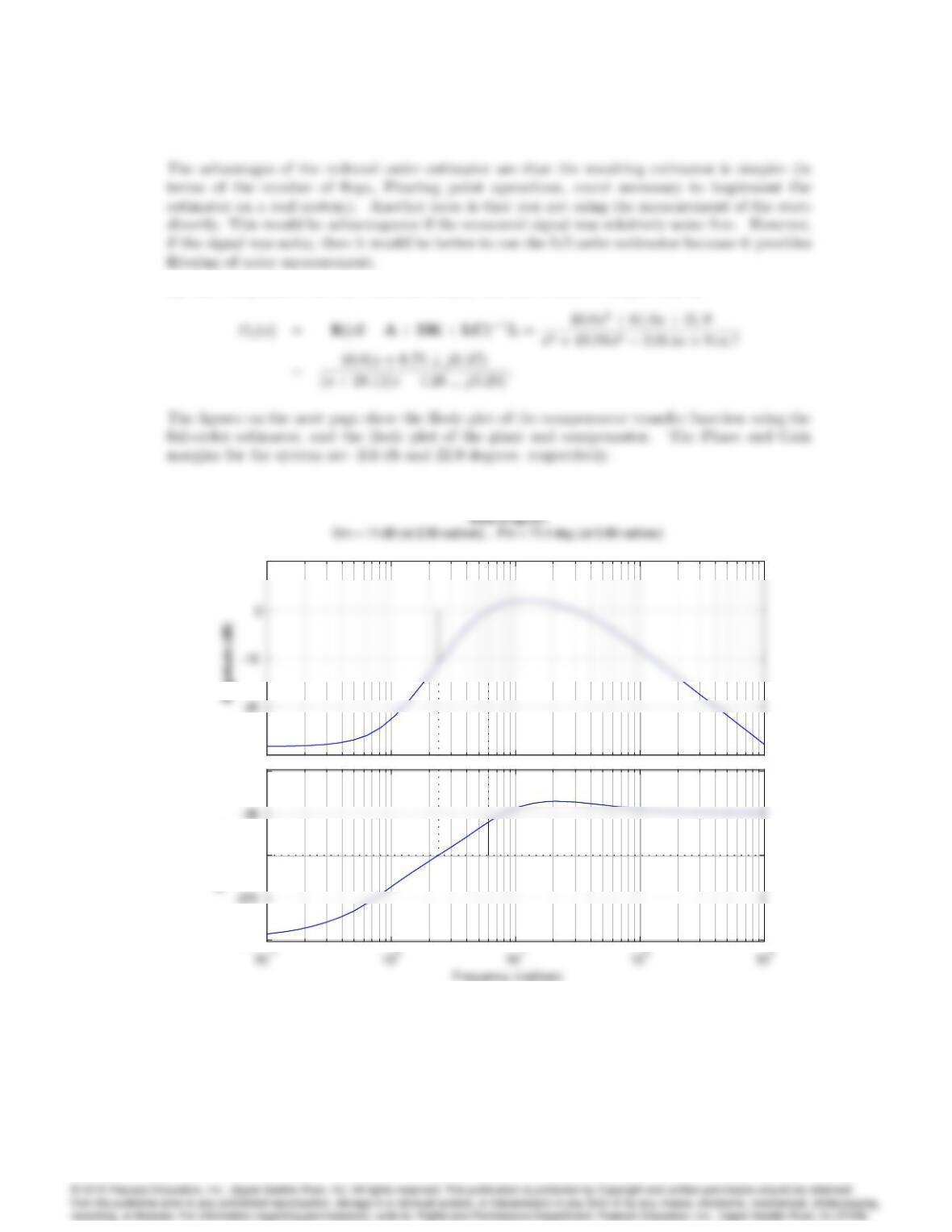
7064 CHAPTER 7. STATE-SPACE DESIGN
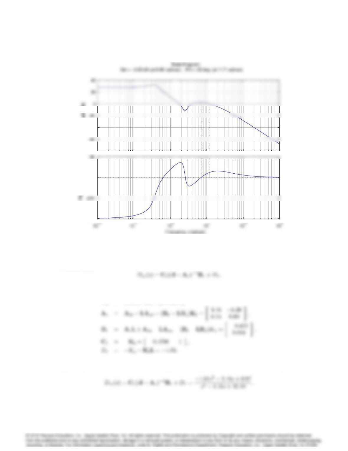
(f) The compensator for the controller in part (c) and estimator in part (d) is,
–30
10
–360
–180
0
Phase (deg)
–30
10
–360
–180
0
Phase (deg)
Problem 7.49: Bode plots of compensator using the full-order estimator alone.
7065
–80
–40
Magnitude (dB)
–360
–180
–80
–40
Magnitude (dB)
–360
–180
Problem 7.49: Bode plot of plant and compensator combined.
(g) Compensator for the controller in part (c) and estimator in part (e) (i.e., the reduced-order
estimator) is,
Ka= 0:0627;Kb= [0:4706;1];
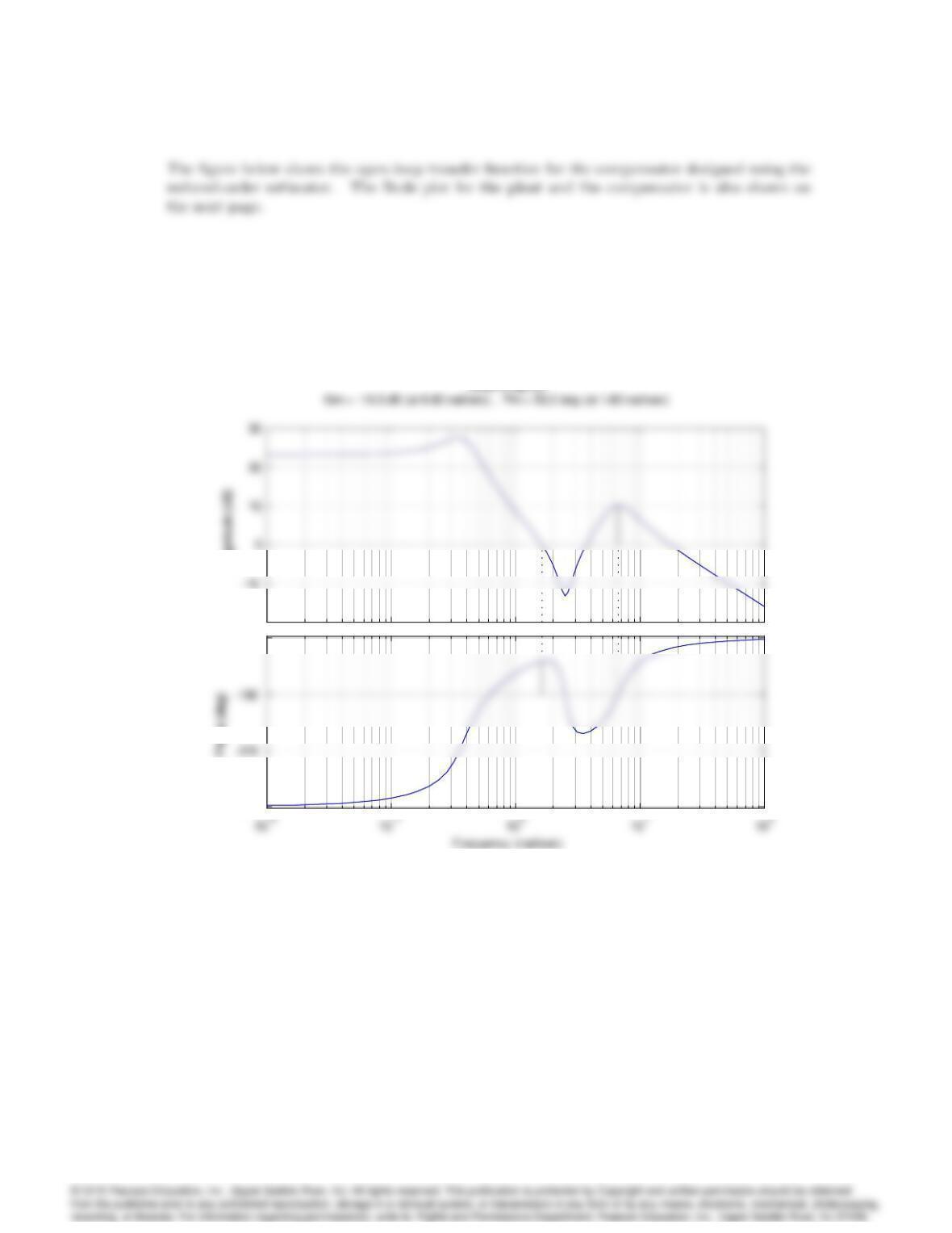
(h) Thus, the transfer function for the compensator using the reduced-order estimator is,
7066 CHAPTER 7. STATE-SPACE DESIGN
–20
Magnitude (dB)
–360
–90
Bode Diag ram
–20
Magnitude (dB)
–360
–90
Problem 7.49: Bode plot of the compensator transfer function using the reduced-order
estimator.
7067
–40
–20
Magnitude (dB)
–360
–180
0
Bode Diag ram
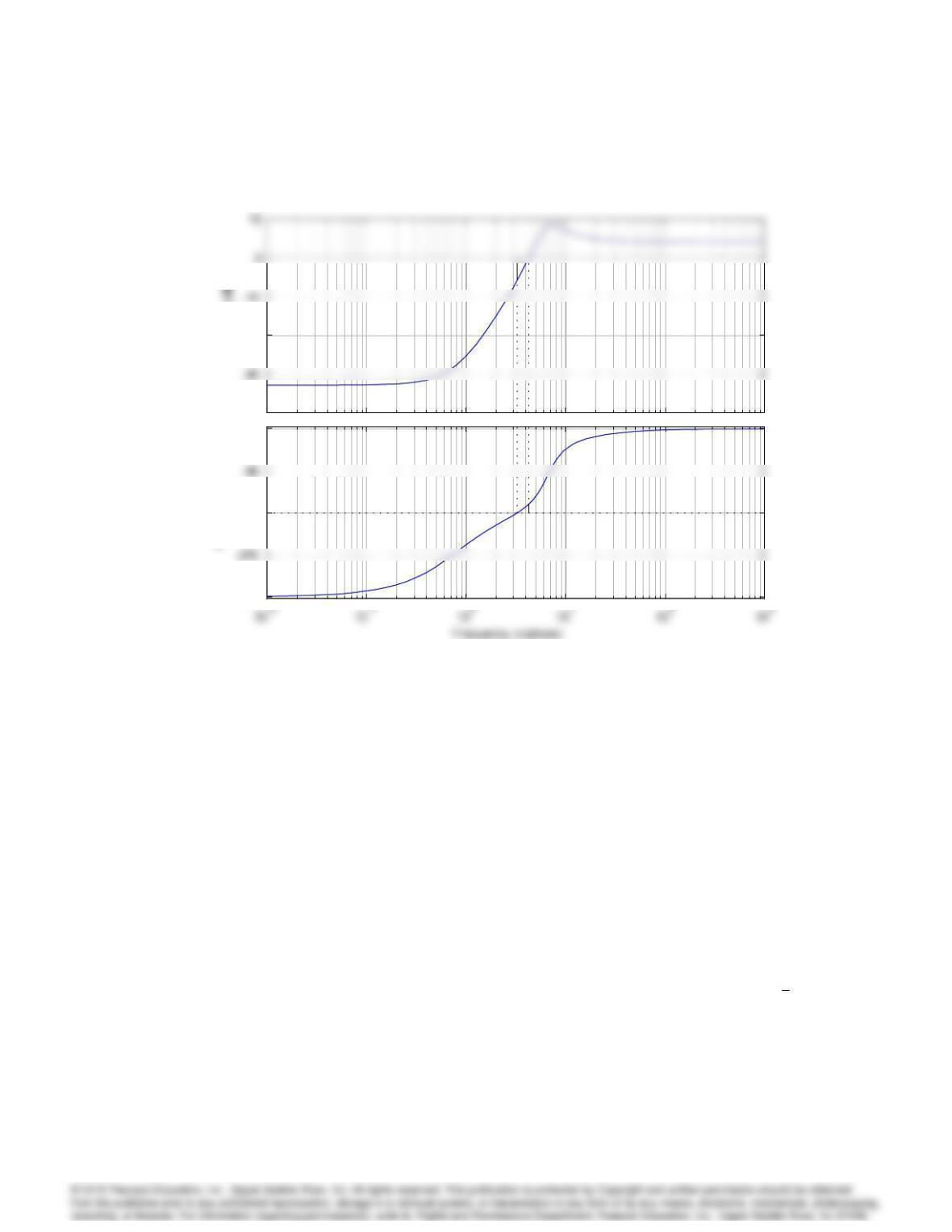
Gm = 5.68 dB (at 3.29 rad/sec) , Pm = 18.5 deg (at 4.28 rad/sec)
–40
–20
Magnitude (dB)
–360
–180
0
Problem 7.49: Bode plot of the compensated system.
50. Suppose a DC drive motor with motor current uis connected to the wheels of a cart in order
to control the movement of an inverted pendulum mounted on the cart. The linearized and
normalized equations of motion corresponding to this system can be put in the form
•
=+v+u;
_v=vu;
where,
= angle of the pendulum;
v= velocity of the cart:
a) We wish to control by feedback to uof the form,
u=K1K2_
K3v:
Find the feedback gains so that the resulting closed-loop poles are located at 1,1jp3.
b) Assume that and vare measured. Construct an estimator for and _
of the form,
_
^x =A^x +L(y^y);
7068 CHAPTER 7. STATE-SPACE DESIGN
where x= [ _
]Tand y=. Treat both vand uas known. Select Lso that the estimator
poles are at 2and 2.
c) Give the transfer function of the controller, and draw the Bode plot of the closed-loop system,
indicating the corresponding gain and phase margins.
d) Using Matlab, plot the response of the system to an initial condition on , and give a
physical explanation for the initial motion of the cart.
Solution:
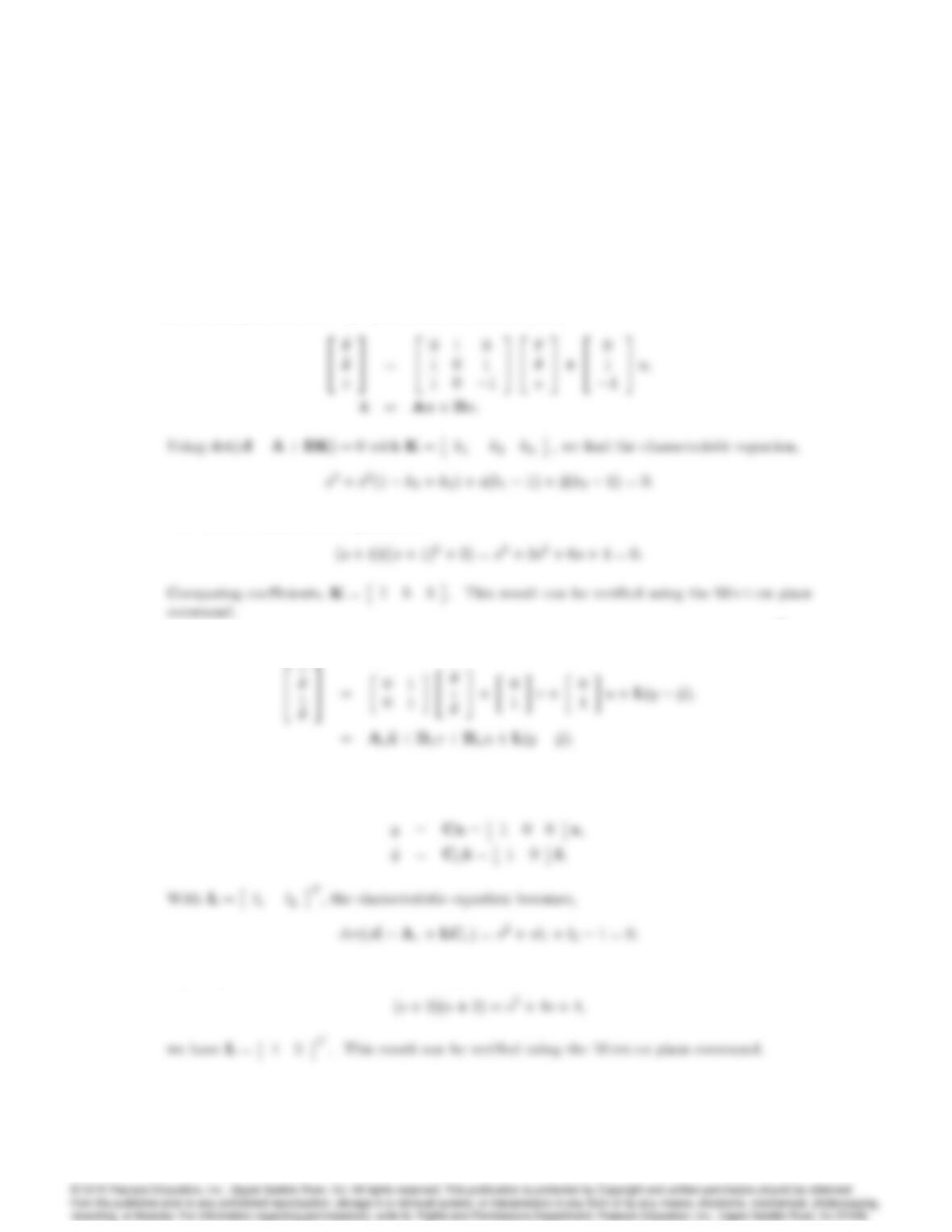
(a) Defining the state x= [ v]T, the system is written as,
The desired characteristic equation is,
(b) The estimator equations (both explicitly and symbolically) for estimating ^x =_
Tare,
2
where uand vare assumed to be known. The output equations for the plant and the estimator
are,
Equating with the desired characteristic equation,
7069
(c) Construct the feedback uin terms of both the measured signal vand the estimated state ^x.
Using the feedback gains from (a), we have,
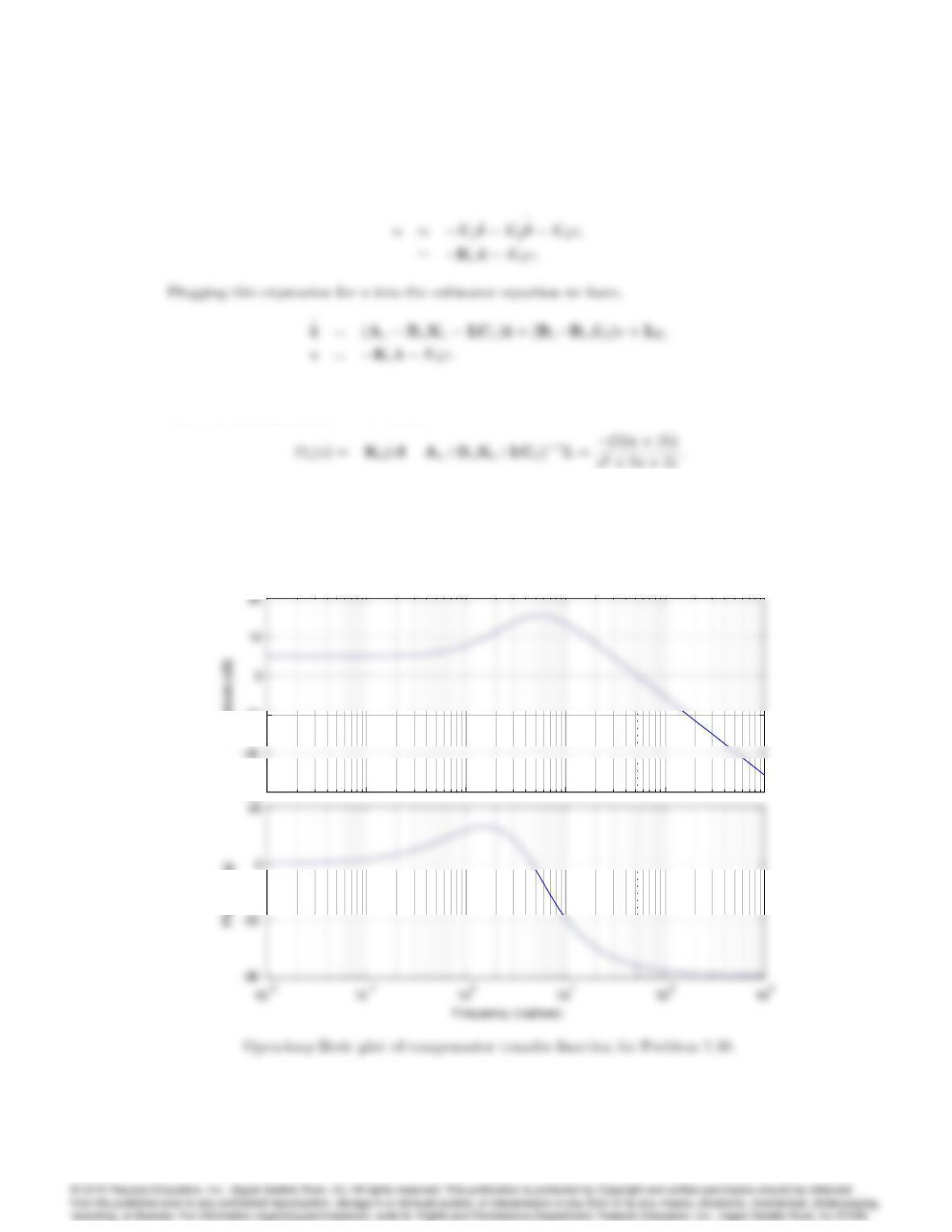
The transfer function from yto ucan now be read directly from these two equations by setting
all of the auxiliary inputs to zero, i.e., v= 0. Thus,
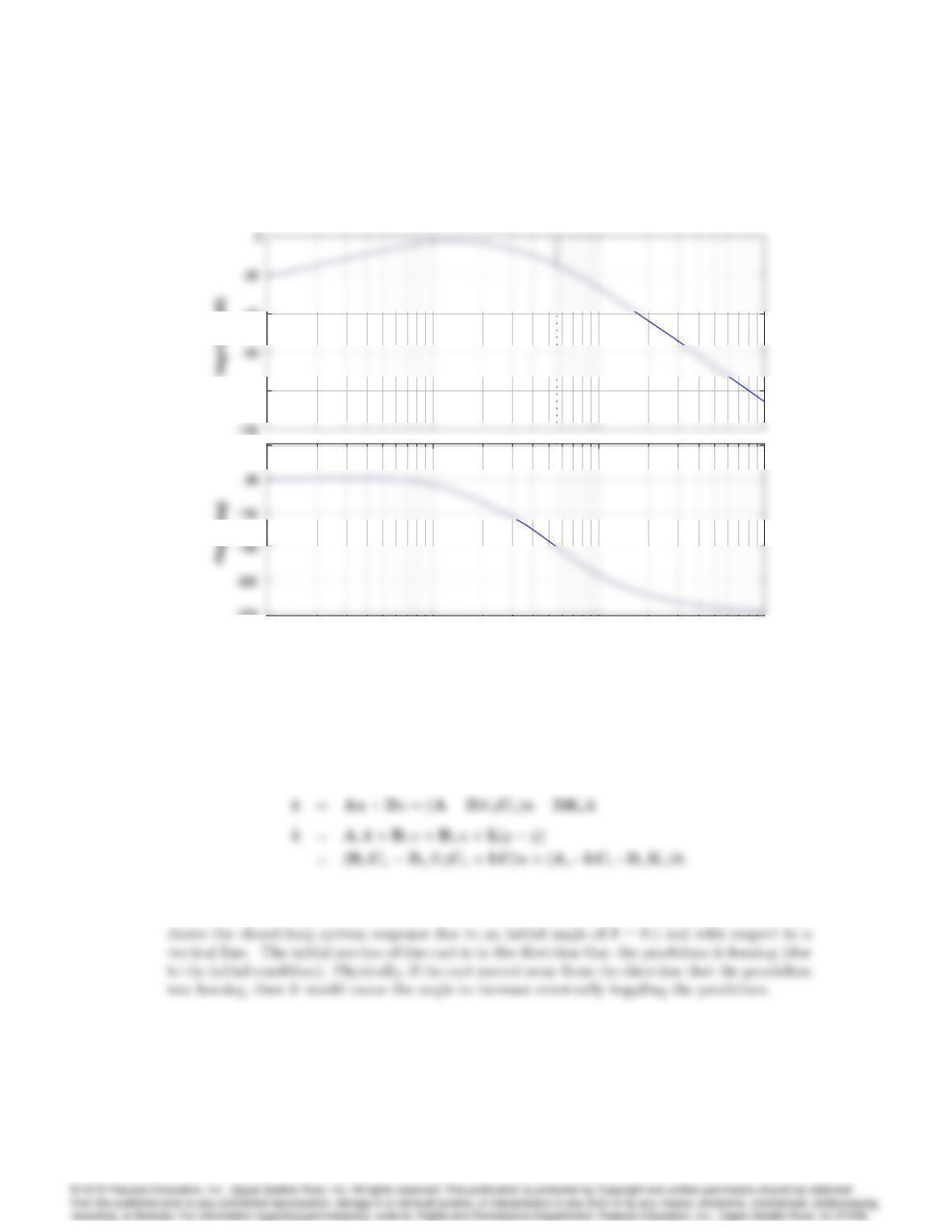
The Bode plots are shown next.
–30
–10
Magnitude (dB)
Bode Diag ram
Gm = Inf , Pm = 98.6 deg (at 52.8 rad/sec)
–30
–10
Magnitude (dB)
7070 CHAPTER 7. STATE-SPACE DESIGN
–80
–40
10
-1
10
0
10
1
10
2
–270
–45
Bode Diag ram
Gm = 14.7 dB (at 5.56 rad/sec) , Pm = Inf
Freq uency (r ad/sec)
–80
–40
10
-1
10
0
10
1
10
2
–270
–45
Bode plot of the compensator and plant together for Problem 7.50.
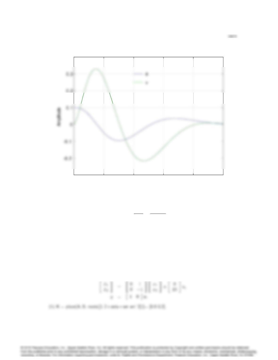
(d) One approach to simulating the system is to augment the plant and estimator equations into
one matrix. Recognizing that v=001x=Cvx, we can eliminate uand v.
This is now easily implemented using the Matlab command lsim. The figure on the next page
0 1 2 3 4 5
–0.3
0.4
Time (sec)
0 1 2 3 4 5
–0.3
0.4
Time (sec)
Angle of pendulum and the velocity of the cart given an initial angle for Problem 7.50.
51. Consider the control of
G(s) = Y(s)
U(s)=10
s(s+ 1):
a) Let y=x1and _x1=x2, and write state equations for the system.
b) Find K1and K2so that u=K1x1K2x2yields closed-loop poles with a natural frequency
!n= 3 and a damping ratio = 0:5.
c) Design a state estimator for the system that yields estimator error poles with !n1= 15 and
1= 0:5.
d) What is the transfer function of the controller obtained by combining parts (a) through (c)?
e) Sketch the root locus of the resulting closed-loop system as plant gain (nominally 10) is varied.
Solution:
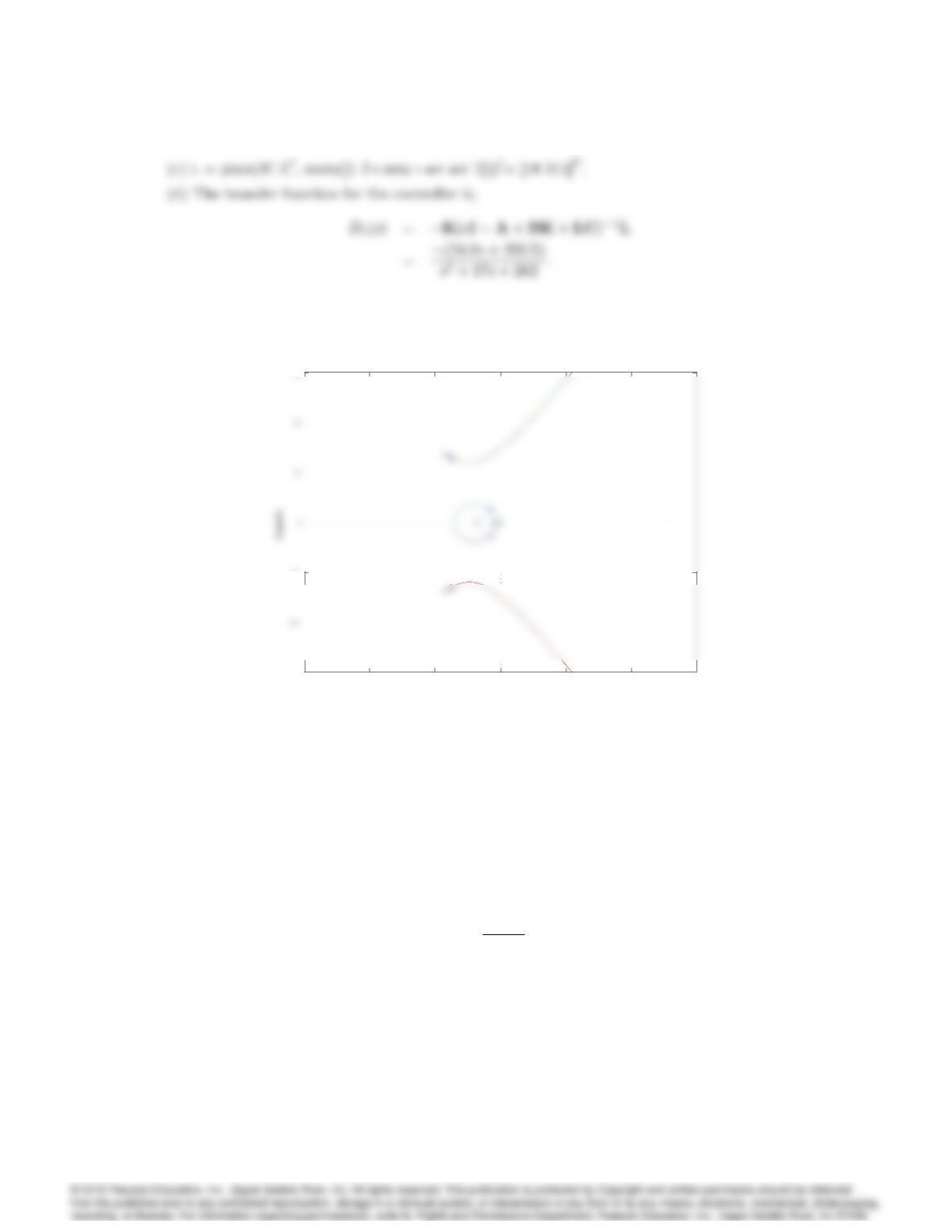
The state equations are,
7072 CHAPTER 7. STATE-SPACE DESIGN
(e) The figure below shows the root locus around a nominal gain of 10, which is indicated by
asterisk.
Root Locus
Real Axis
-30 -20 -10 010 20 30
-30
-10
30
Problem 7.51: Root locus of the closed-loop system as plant gain is varied.
52. Unstable equations of motion of the form,
•x=x+u;
arise in situations where the motion of an upside-down pendulum (such as a rocket) must be
controlled.
a) Let u=Kx (position feedback alone), and sketch the root locus with respect to the scalar
gain K.
b) Consider a lead compensator of the form,
U(s) = Ks+a
s+ 10X(s):
Select aand Kso that the system will display a rise time of about 2 sec and no more than 25%
overshoot. Sketch the root locus with respect to K.
c) Sketch the Bode plot (both magnitude and phase) of the uncompensated plant.
d) Sketch the Bode plot of the compensated design, and estimate the phase margin.
e) Design state feedback so that the closed-loop poles are at the same locations as those of the
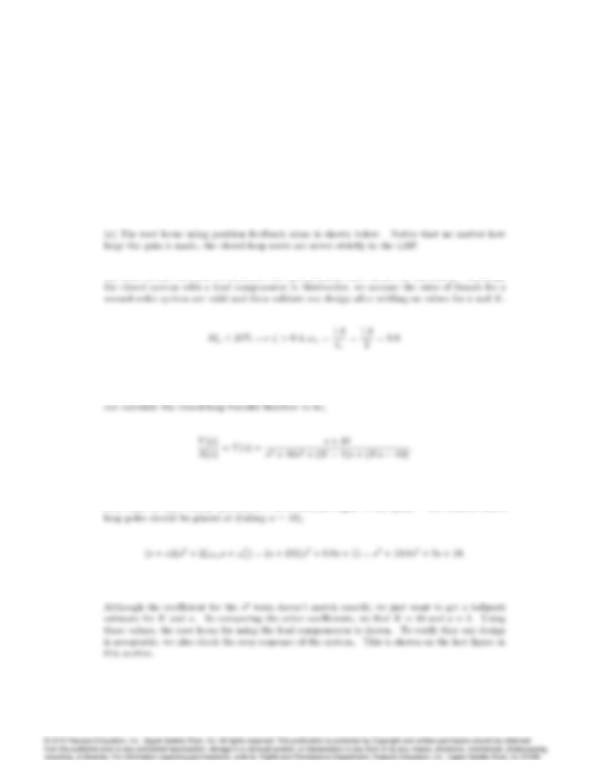
7073
design in part (b).
f) Design an estimator for xand _xusing the measurement of x=y, and select the observer gain
Lso that the equation for ~xhas characteristic roots with a damping ratio = 0:5and a natural
frequency !n= 8 rad/sec.
g) Draw a block diagram of your combined estimator and control law, and indicate where ^xand
_xappear. Draw a Bode plot for the closed-loop system, and compare the resulting bandwidth
and stability margins with those obtained using the design of part (b).
Solution:
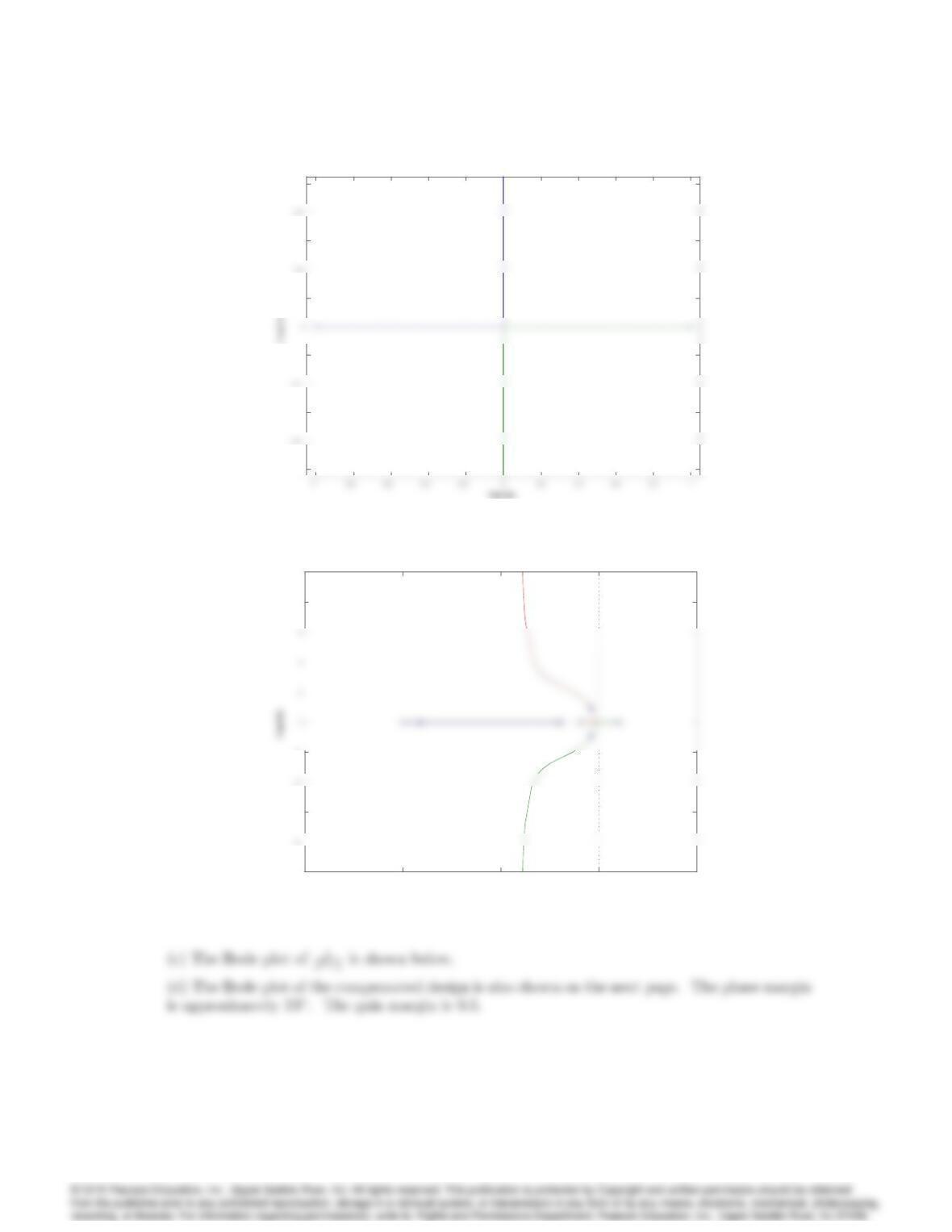
(b) First of all, we need to translate the specifications into values for !nand . Although
Try = 0:4and !n= 1 for the design. Because the form of the compensator is specified, we
Note that we have subtly introduced ras a reference input to the plant. The desired closed
7074 CHAPTER 7. STATE-SPACE DESIGN
Root Locus
-1
-0.6
-0.2
0.2
0.6
1
Problem 7.52: Root locus with position feedback alone.
Root Locus
Real Axis
-15 -10 -5 0 5
-10
-6
-2
8
10
Root locus for Problem 7.52.
7075
–40
–20
0
-1
0
1
–181
–180
–179
–40
–20
0
-1
0
1
–181
–180
–179
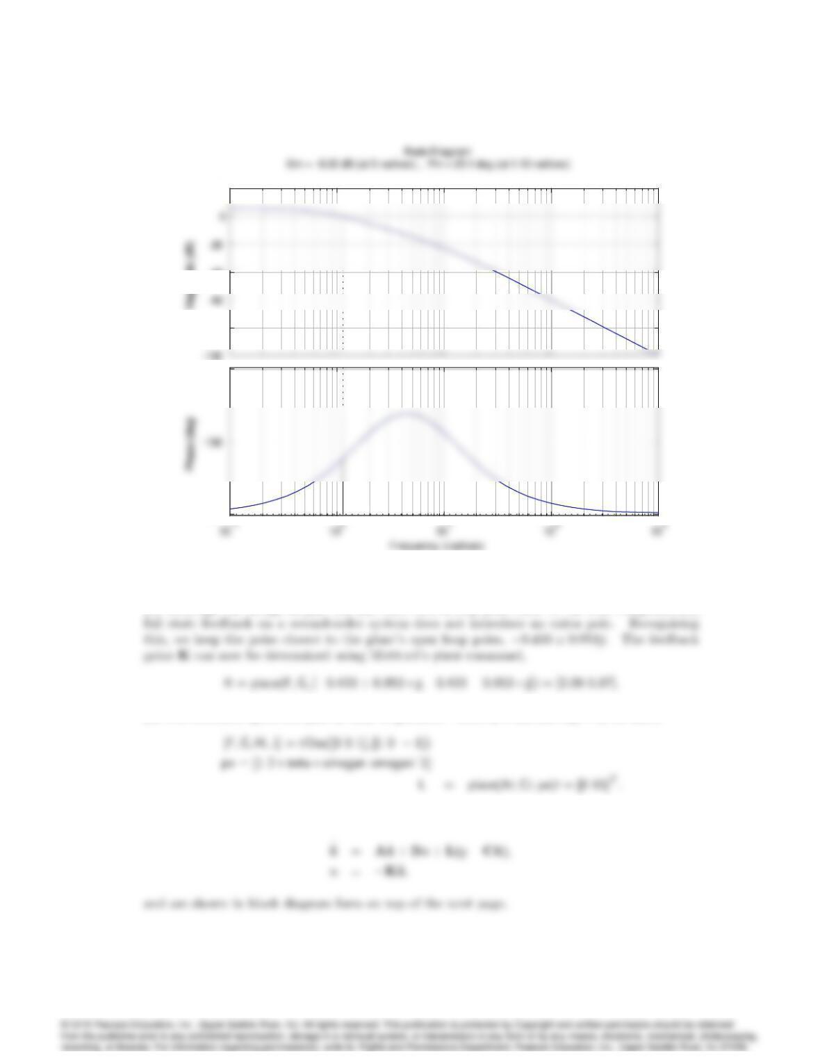
Problem 7.52: Bode plots for the open-loop system.
7076 CHAPTER 7. STATE-SPACE DESIGN
–80
–40
20
–180
–120
–80
–40
20
–180
–120
Problem 7.52: Compensator and plant combined.
(e) Although the design in part (b) has three closed-loop poles (due to the lead compensator),
(f) The estimator gains are just as easy to produce. With = 0:5and !n= 8, we have,
(g) The estimator equations are,
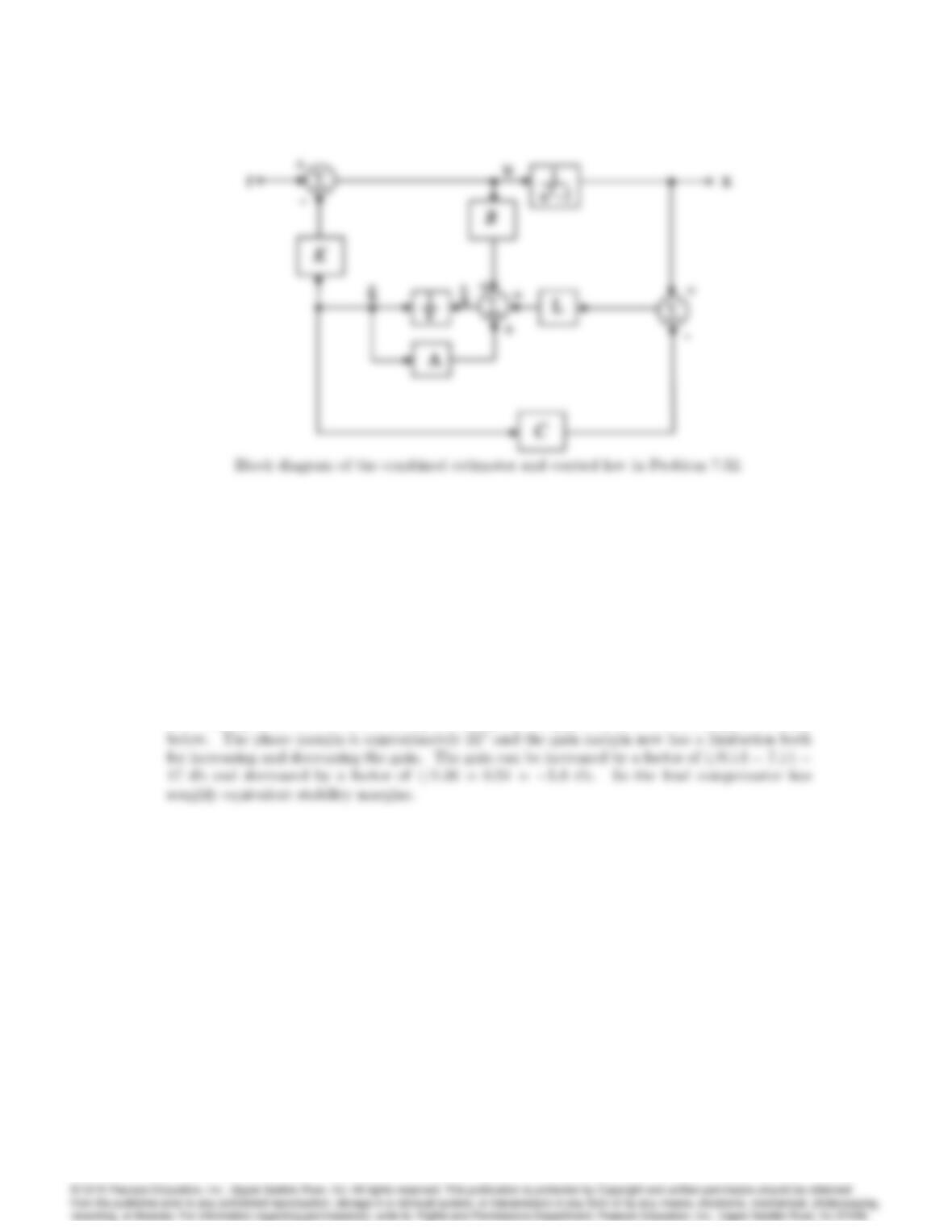
7077
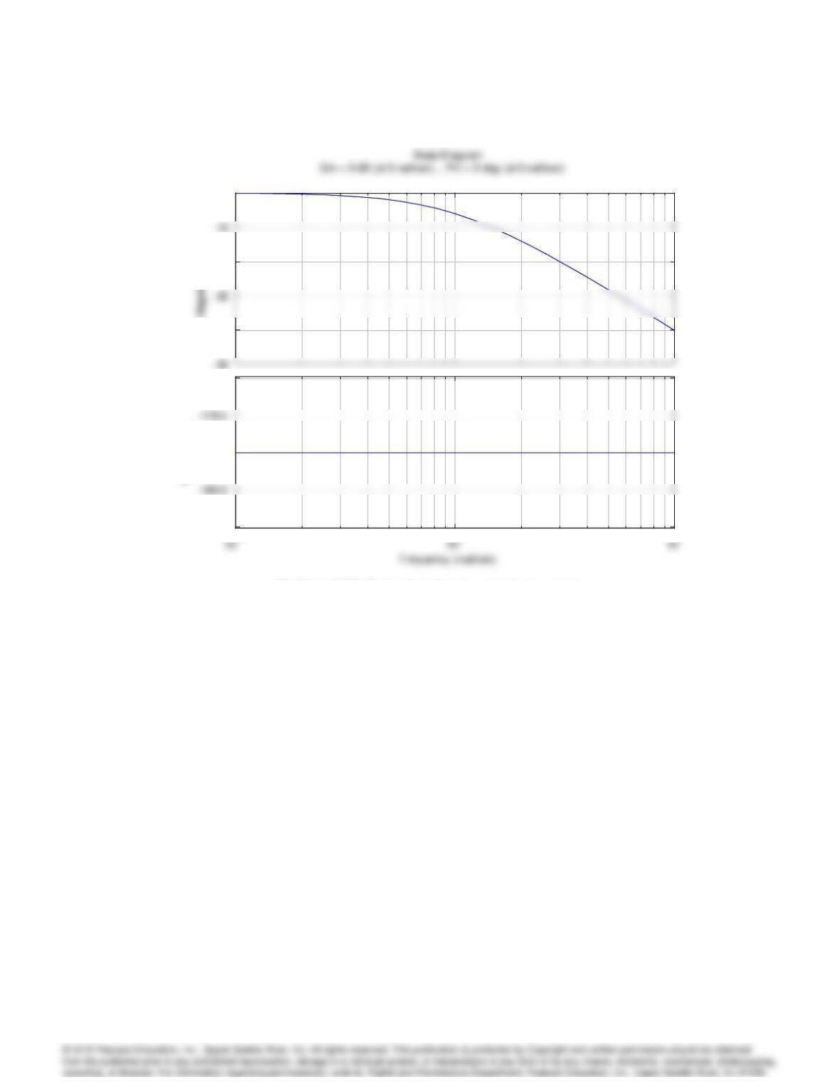
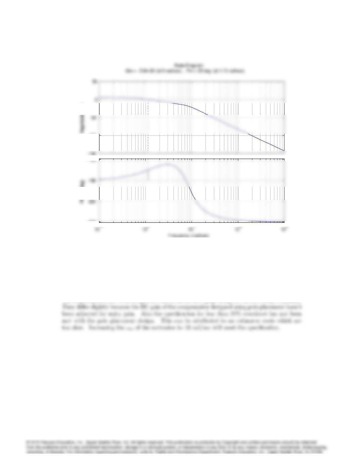
The Bode plot of the controller and plant designed using pole placement techniques is shown
7078 CHAPTER 7. STATE-SPACE DESIGN
–100
–270
–100
–270
Problem 7.52: Bode plot of plant and compensator design with pole placement.
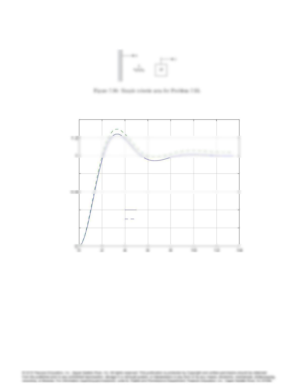
The step responses for both designs are shown on the next page using the Matlab step command.
7079
0.2
0.4
0.8
1.4
Lead design
Pole placement design
0.2
0.4
0.8
1.4
Lead design
Pole placement design
Problem 7.52: Closed-loop step responses.
53. A simplified model for the control of a ‡exible robotic arm is shown in Fig. 7.98, where
k=M = 900 rad=sec2;
y= output;the mass position;
u= input;the position of the end of the spring:
a) Write the equations of motion in state-space form.
b) Design an estimator with roots as s=100 100j.