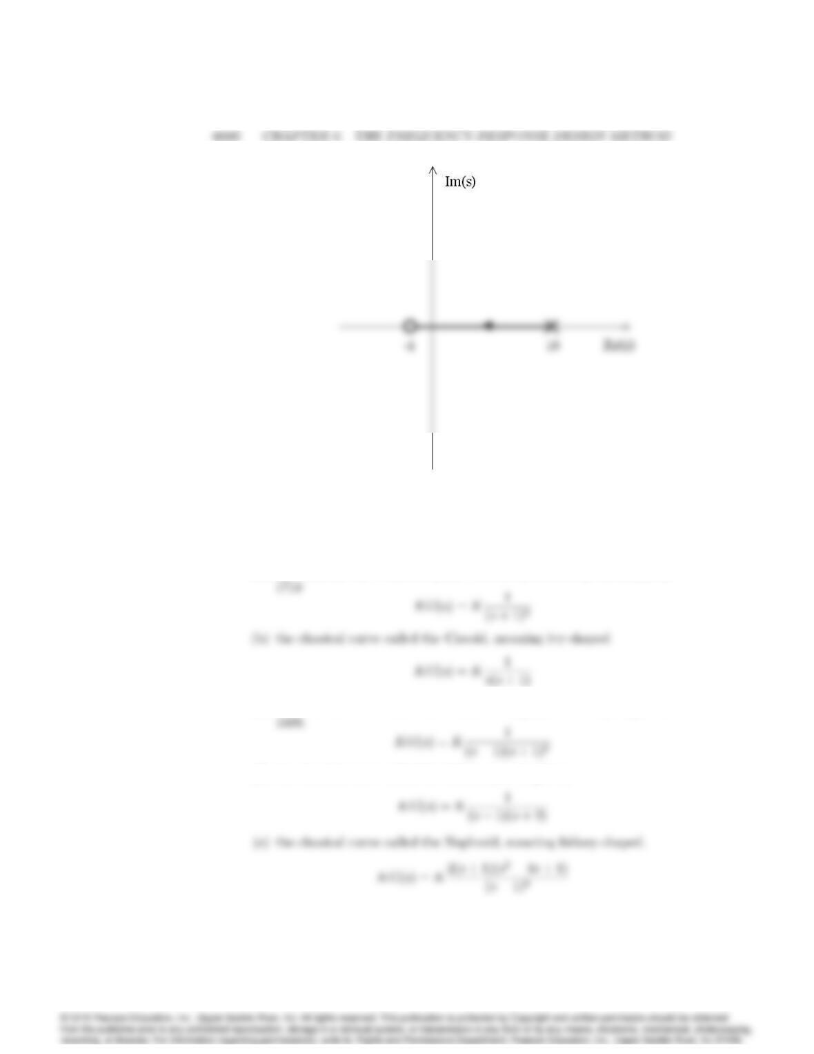
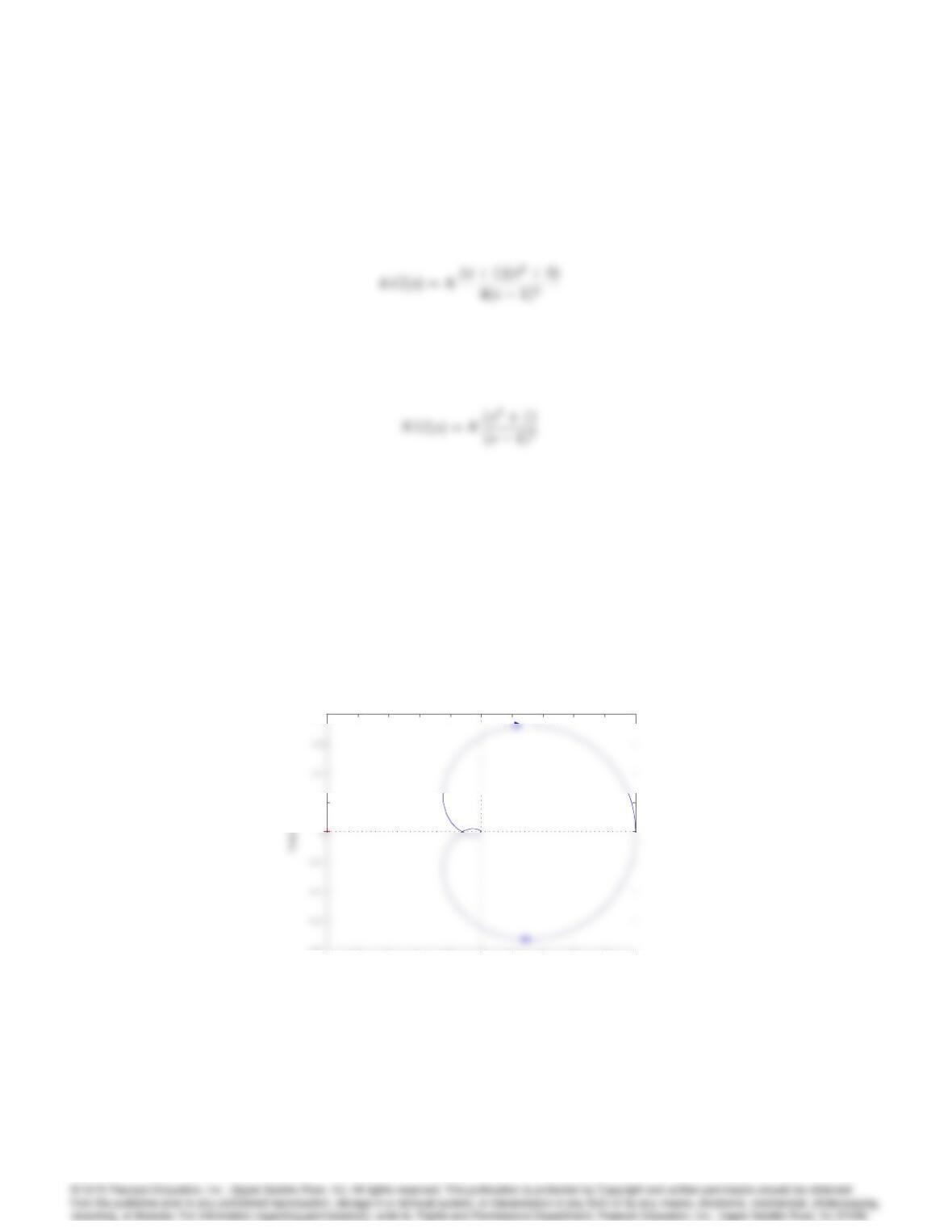
23. Nyquist plots and their classical plane curves: Determine the Nyquist plot
using Matlab for the systems given below with K= 1 and verify that
the beginning point and end point for the j! > 0portion have the correct
magnitude and phase:
(a) the classical curve called Cayley’s Sextic, discovered by Maclaurin in
(c) the classical curve called the Folium of Kepler, studied by Kepler in
(d) the classical curve called the Folium (not Kepler’s)
6081
(f) the classical curve called Nephroid of Freeth, named after the English
mathematician T. J. Freeth.
(g) a shifted Nephroid of Freeth
Solution :
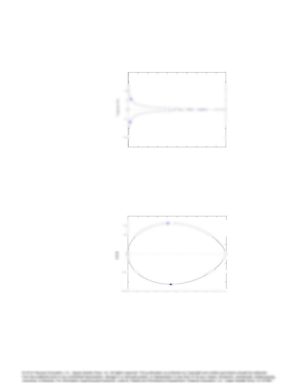
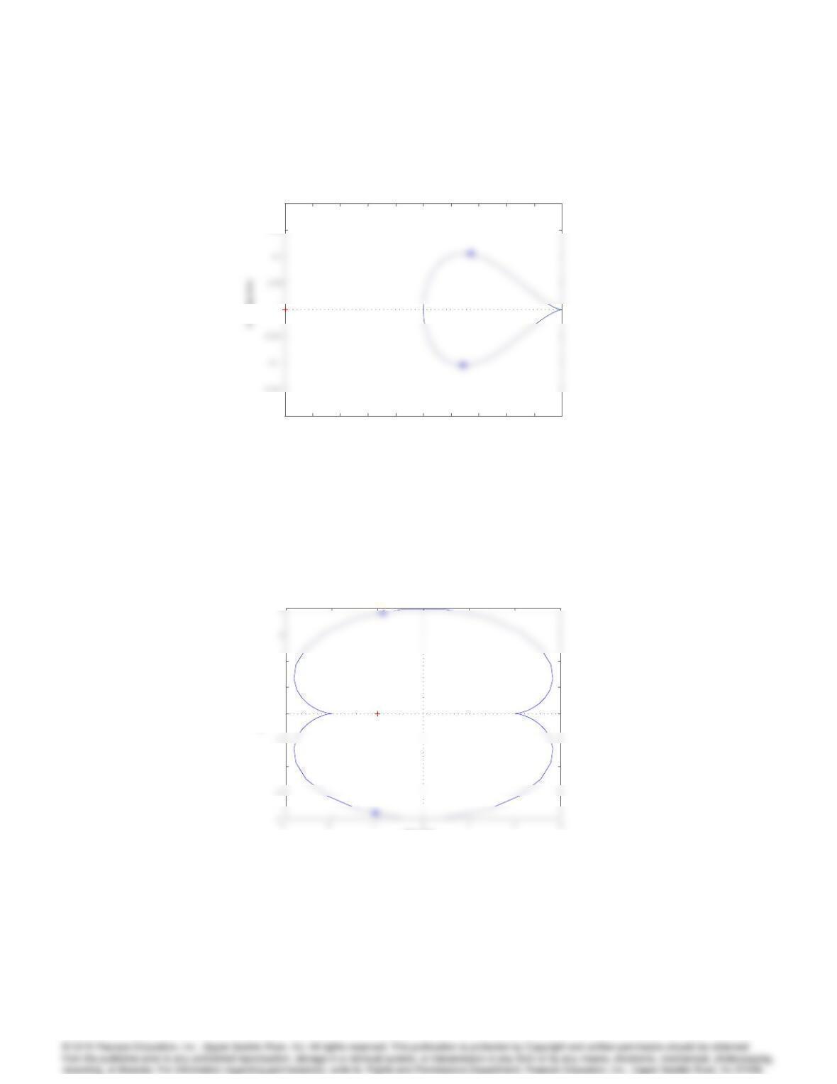
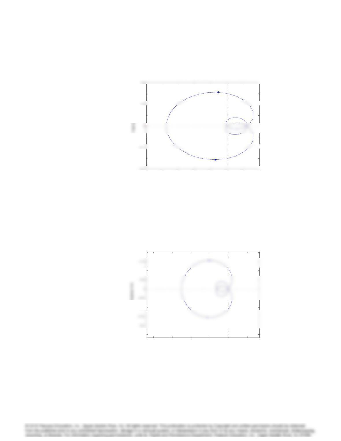
These are all accomplished by using Matlab’s Nyquist function. All
interesting shapes. To check the magnitude and phase for each,
plug in s= 0 and s= inf and then compare those values with the
beginning and end points on the Nyquist diagrams.
(a)
-1 -0.8 -0.6 -0.4 -0.2 00.2 0.4 0.6 0.8 1
-0.8
0.2
0.8
Nyquist Diagram
Real Axis
(b)
6082 CHAPTER 6. THE FREQUENCY-RESPONSE DESIGN METHOD
-1 –0.9 –0.8 -0.7 –0.6 -0.5 -0.4 -0.3 -0.2 -0.1 0
–20
–10
15
20
Nyquist Diagram
Real Axis
(c)
-1 –0.9 -0.8 -0.7 –0.6 -0.5 -0.4 -0.3 –0.2 –0.1 0
–0.3
–0.1
0.1
0.4
Nyquist Diagram
Real Axis
(d)
6083
-1 –0.9 -0.8 -0.7 –0.6 –0.5 -0.4 -0.3 –0.2 -0.1 0
–0.2
0
0.15
0.2
Nyquist Diagram
Real Axis
(e)
-2
0
1
2
Nyquist Diagram
Real Axis
Imaginary Axis
(f)
6084 CHAPTER 6. THE FREQUENCY-RESPONSE DESIGN METHOD
-1 –0.8 -0.6 –0.4 -0.2 0 0.2 0.4
–0.6
–0.2
0.2
0.6
Nyquist Diagram
Real Axis
(g)
–0.4 -0.3 -0.2 -0.1 0 0.1
–0.25
–0.1
0.1
0.2
Nyquist Diagram
Real Axis
Imaginary Axis
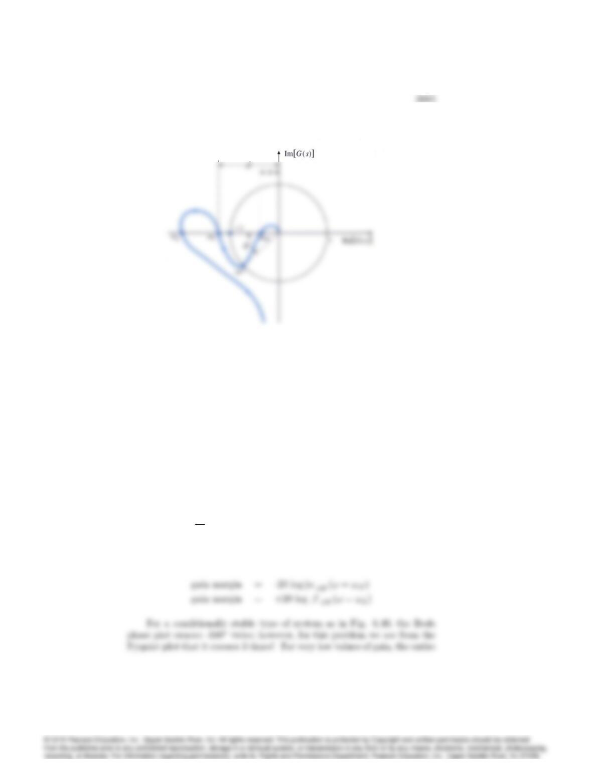
Figure 6.88: Nyquist plot for Problem 24
(a) Problems and Solutions for Section 6.4
24. The Nyquist plot for some actual control systems resembles the one shown
in Fig.6.88. What are the gain and phase margin(s) for the system of
Fig. 6.88 given that = 0:4; = 1:3;and = 40o:Describe what
happens to the stability of the system as the gain goes from zero to a very
large value. Sketch what the corresponding root locus must look like for
such a system. Also sketch what the corresponding Bode plots would look
like for the system.
Solution :
The phase margin is defined as in Figure 6.34, P M =(!=!),
but now there are several gain margins! If the system gain is increased
(multiplied) by 1
jjor decreased (divided) by jj, then the system will go
unstable. This is a conditionally stable system. See Figure 6.40 for a
typical root locus of a conditionally stable system.
6086 CHAPTER 6. THE FREQUENCY-RESPONSE DESIGN METHOD
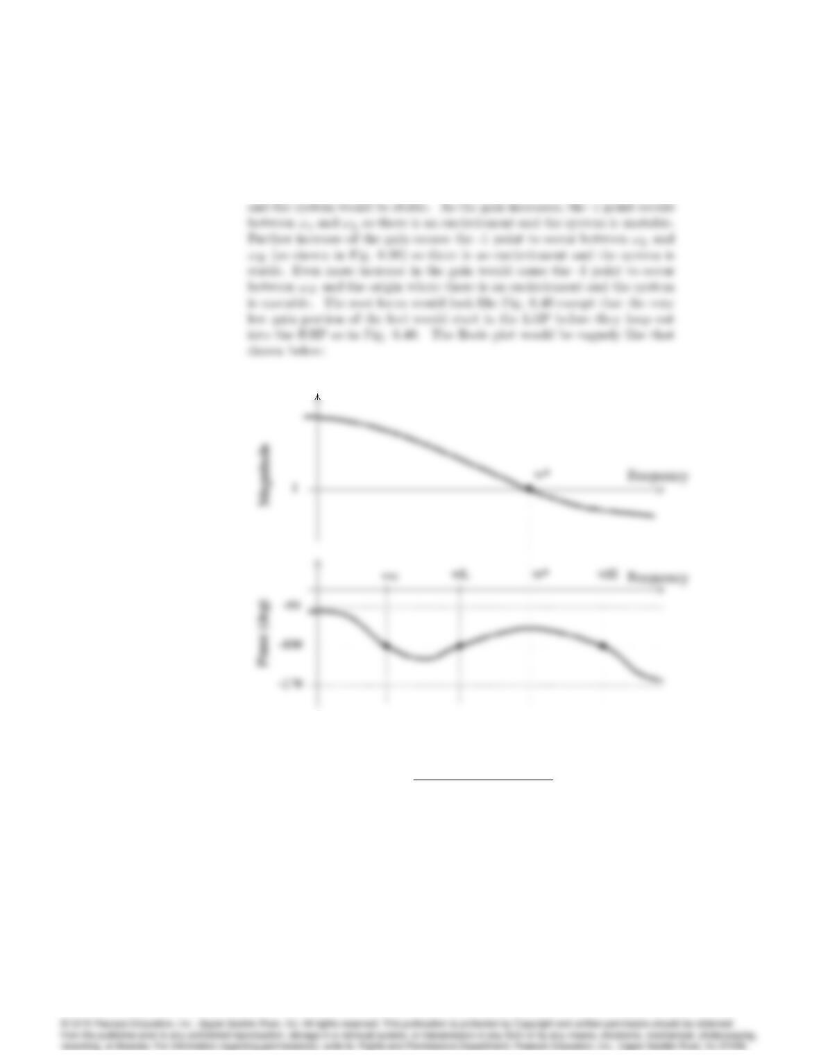
Nyquist plot would be shrunk, and the -1 point would occur to the left of
the negative real axis crossing at !o, so there would be no encirclements
25. The Bode plot for
G(s) = 100[(s=10) + 1]
s[(s=1) 1][(s=100) + 1]
is shown in Fig. 6.89.
(a) Why does the phase start at -270oat the low frequencies?
(b) Sketch the Nyquist plot for G(s).
(c) Is the closed-loop system shown in Fig. 6.89 stable?
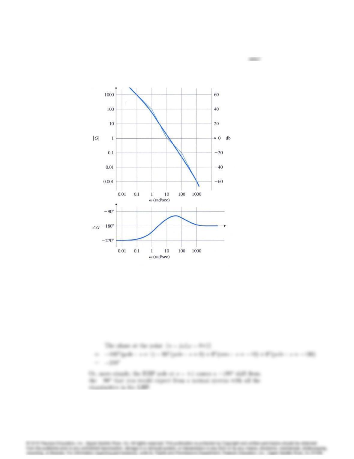
Figure 6.89: Bode plot for Problem 25
(d) Will the system be stable if the gain is lowered by a factor of 100?
Make a rough sketch of a root locus for the system and qualitatively
confirm your answer
Solution :
(a) From the root locus, the phase at the low frequencies (!= 0+) is
calculated as :
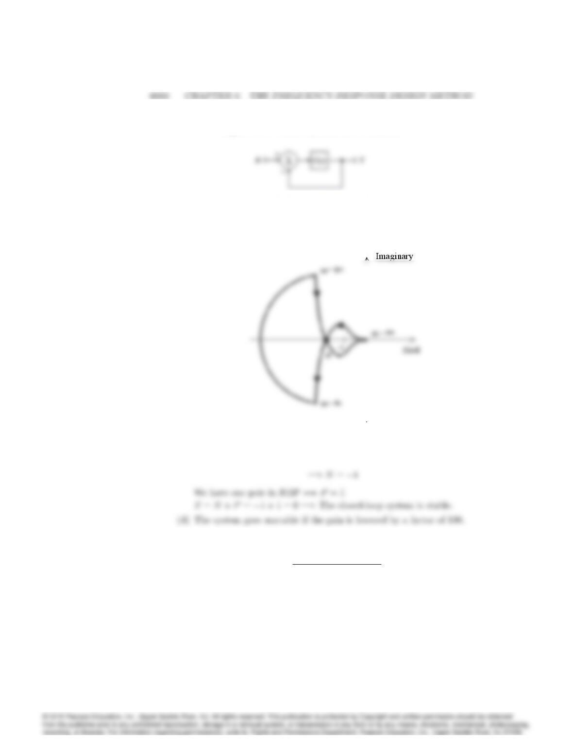
Figure 6.90: Control system for Problem 26
(b) The Nyquist plot for G(s):
(c) As the Nyquist shows, there is one counter-clockwise encirclement of
-1.
26. Suppose that in Fig. 6.90,
G(s) = 25(s+ 1)
s(s+ 2)(s2+ 2s+ 16):
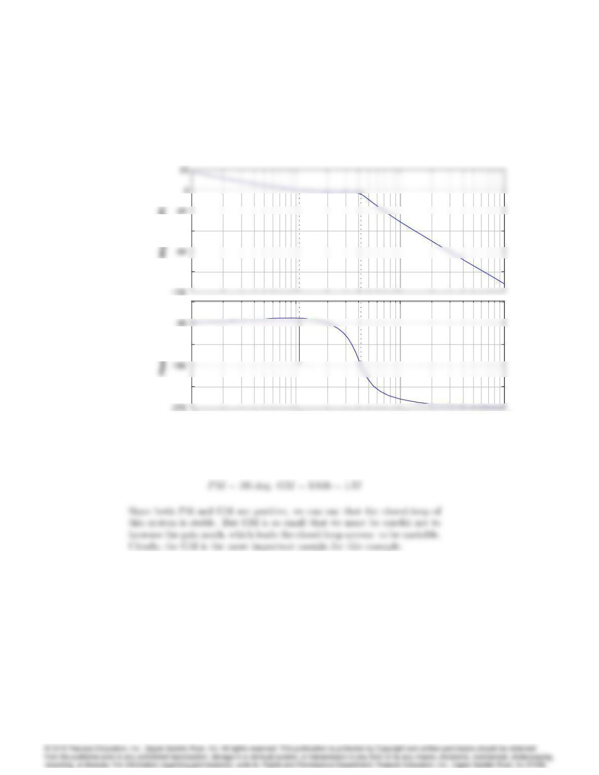
Use MATLAB’s margin to calculate the PM and GM for G(s)and, based
on the Bode plots, conclude which margin would provide more useful in-
formation to the control designer for this system.
Solution :
6089
–80
–40
10
-1
10
0
10
1
10
2
–225
–135
–45
Bode Diagram
Gm = 3.91 dB (at 4.22 rad/sec) , Pm = 101 deg (at 1.08 rad/sec)
Frequency (rad/sec)
–80
–40
10
-1
10
0
10
1
10
2
–225
–135
–45
From the Bode plot,
27. Consider the system given in Fig. 6.91.
(a) Use MATLAB to obtain Bode plots for K= 1 and use the plots to
estimate the range of Kfor which the system will be stable.
(b) Verify the stable range of Kby using margin to determine PM for
selected values of K.
(c) Use rlocus and rlocfind to determine the values of Kat the stability
boundaries.
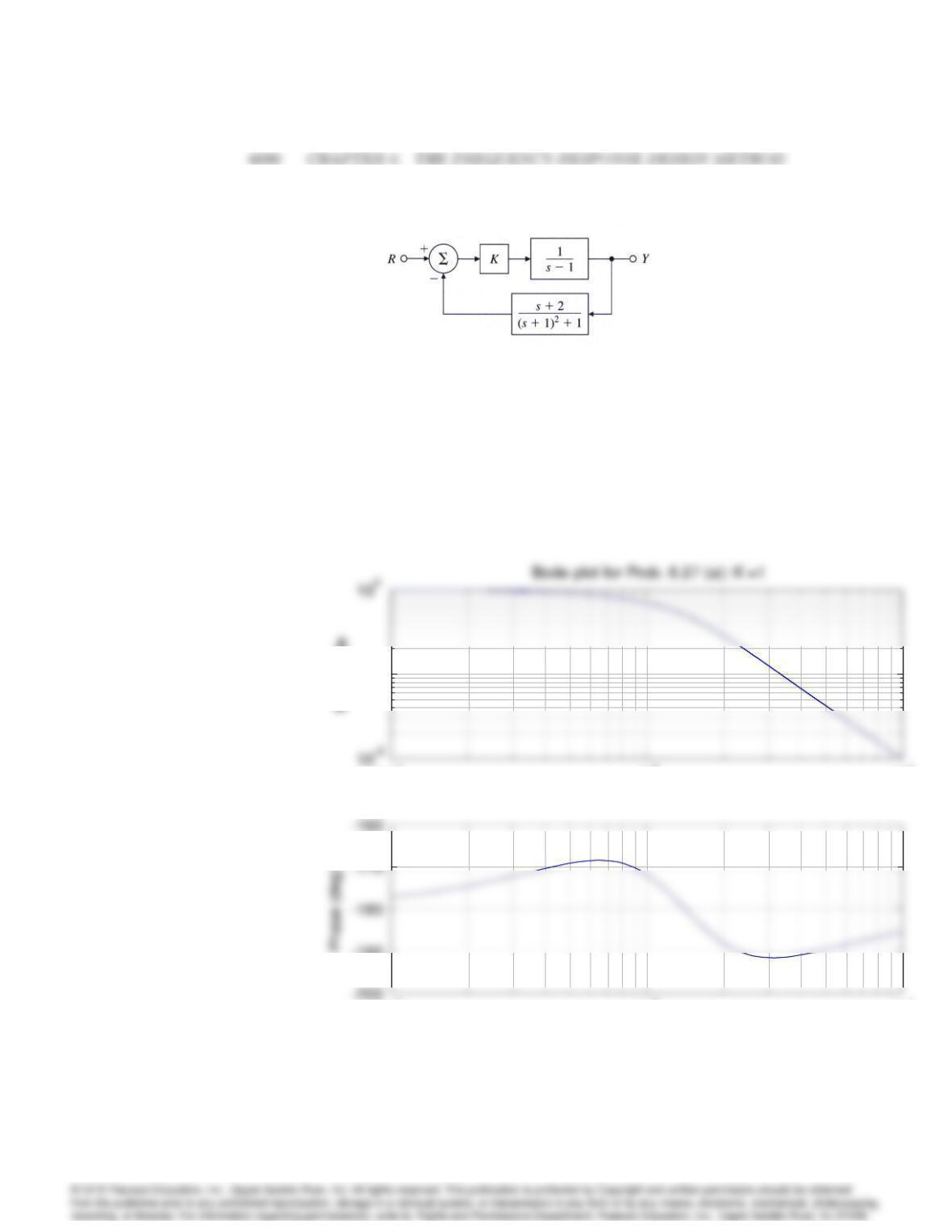
Figure 6.91: Control system for Problem 27
(d) Sketch the Nyquist plot of the system, and use it to verify the number
of unstable roots for the unstable ranges of K.
(e) Using Routh’s criterion, determine the ranges of Kfor closed-loop
stability of this system.
Solution :
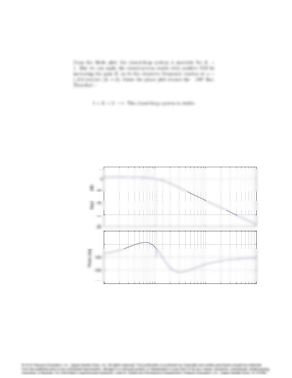
(a) The Bode plot for K= 1 is :
10-1 100101
10-1
Frequency (rad/sec)
10-1 100101
10-1
Frequency (rad/sec)
10-1 100101
-190
ω (rad/sec)
10-1 100101
10-1
Frequency (rad/sec)
10-1 100101
10-1
Frequency (rad/sec)
10-1 100101
-190
ω (rad/sec)
6091
(b) For example, P M = 6:66 deg for K= 1:5.
–20
20
10
-1
10
0
10
1
10
2
–200
–170
–160
Bode Diagram
Gm = 2.5 dB (at 1.41 rad/sec) , Pm = 6.66 deg (at 1.08 rad/sec)
Frequency (rad/sec)
–20
20
10
-1
10
0
10
1
10
2
–200
–170
–160
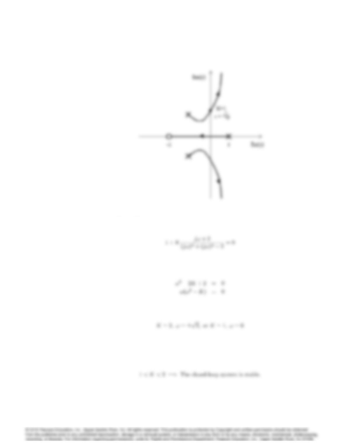
(c) Root locus is :
6092 CHAPTER 6. THE FREQUENCY-RESPONSE DESIGN METHOD
j!-crossing :
Therefore,
6093
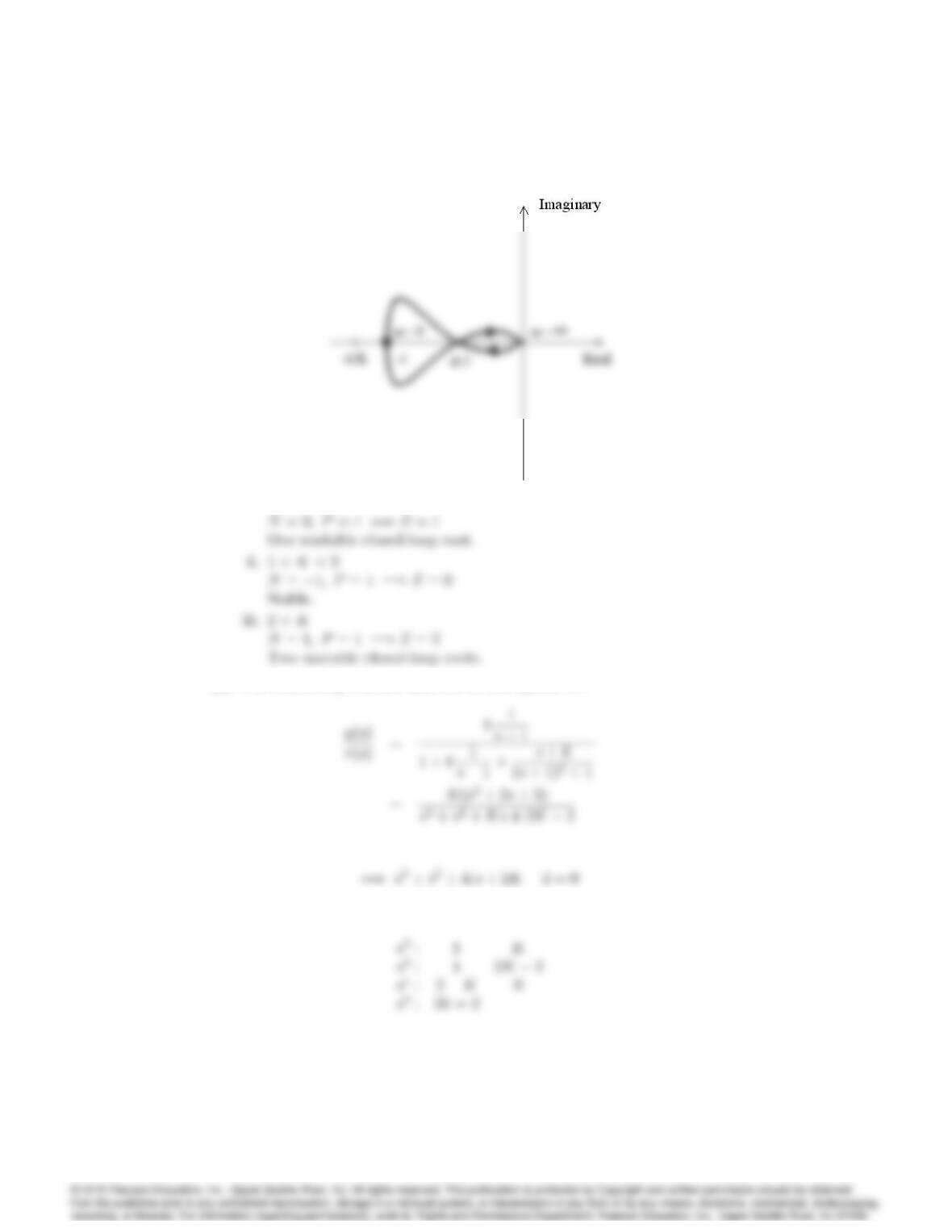
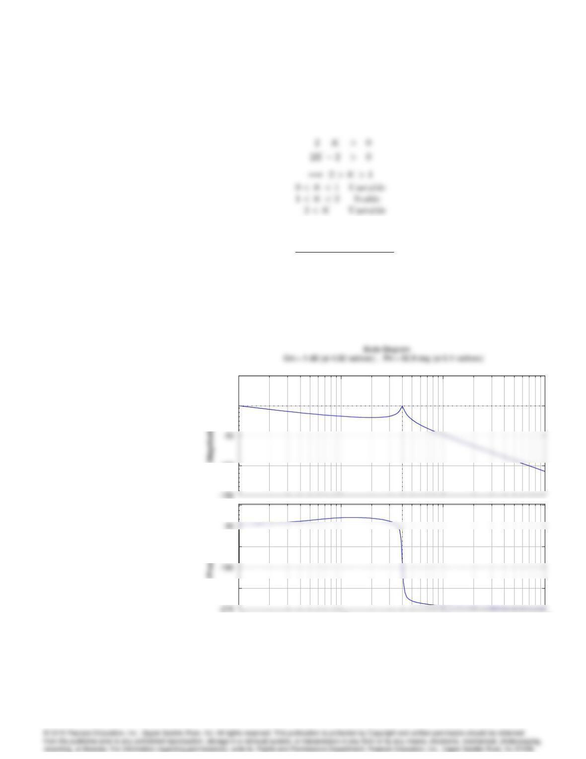
(d)
i. 0< K < 1
(e) The closed-loop transfer function of this system is :
So the characteristic equation is :
Using the Routh’s criterion,
For stability,
6094 CHAPTER 6. THE FREQUENCY-RESPONSE DESIGN METHOD
28. Suppose that in Fig. 6.90,
G(s) = 3:2(s+ 1)
s(s+ 2)(s2+ 0:2s+ 16):
Use MATLAB’s margin to calculate the PM and GM for G(s)and comment
on whether you think this system will have well damped closed-loop roots.
Solution :
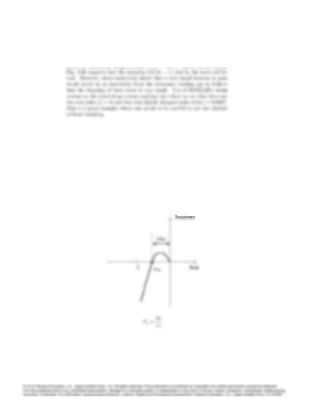
MATLAB’s margin plot for the given system is :
–100
0
50
10
-1
10
0
10
1
10
2
–225
–135
–45
Frequency (rad/sec)
–100
0
50
10
-1
10
0
10
1
10
2
–225
–135
–45
6095
29. For a given system, show that the ultimate period Puand the correspond-
ing ultimate gain Kufor the Zeigler-Nichols method can be found using
the following:
(a) Nyquist diagram
(b) Bode plot
(c) root locus.
Solution :
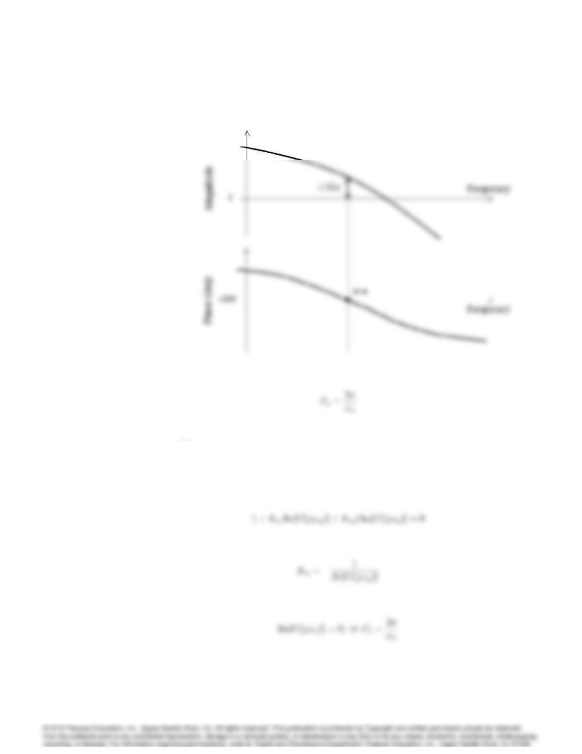
(a) See sketch below.
(b) See sketch below.
6096 CHAPTER 6. THE FREQUENCY-RESPONSE DESIGN METHOD
(c)
1 + KuG(j!u) = 0
30. If a system has the open-loop transfer function
with unity feedback, then the closed-loop transfer function is given by
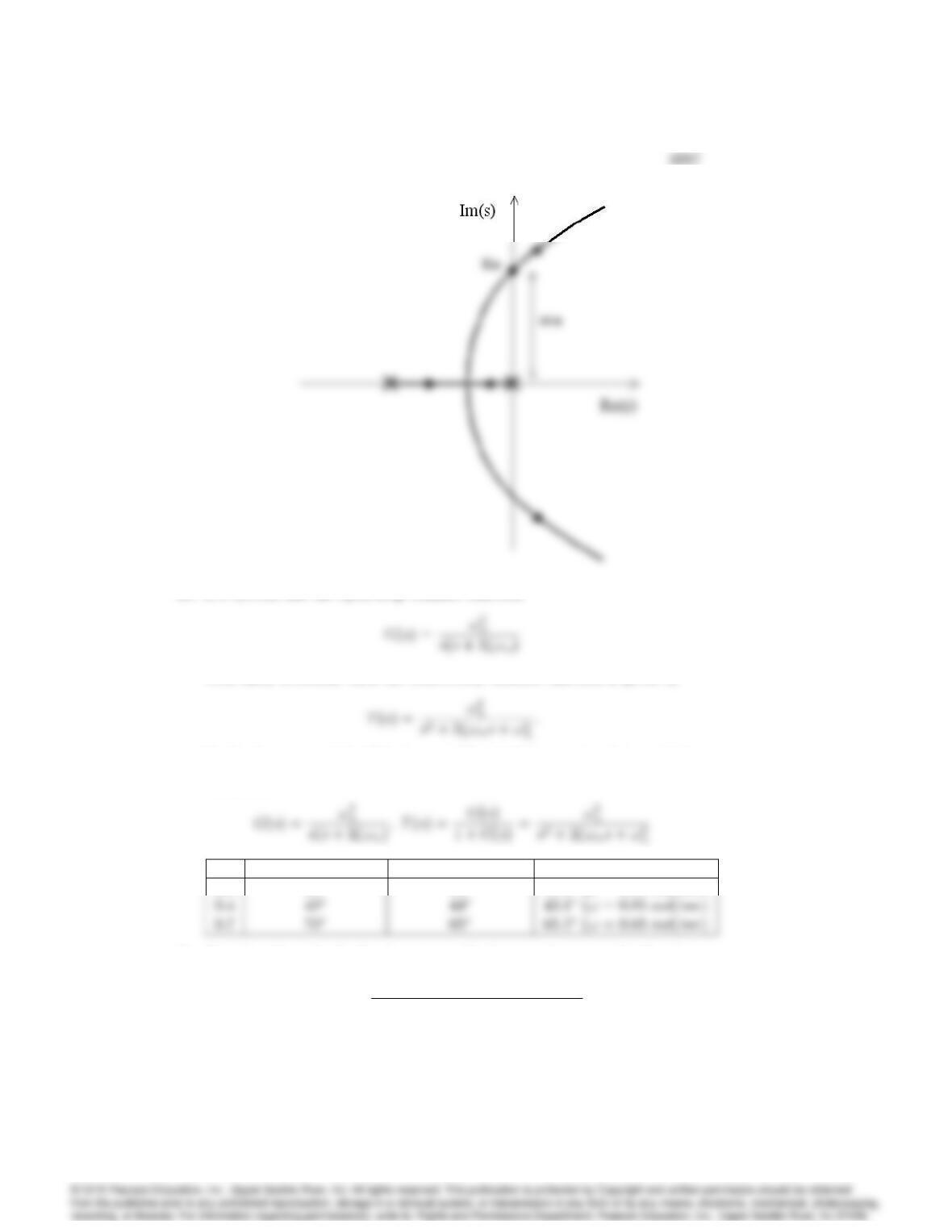
Verify the values of the PM shown in Fig. 6.36 for = 0:1, 0.4, and 0.7.
Solution :
PM from Eq. 6.32 PM from Fig. 6.36 PM from Bode plot
0.1 101011.4(!= 0:99 rad/sec)
31. Consider the unity feedback system with the open-loop transfer function
G(s) = K
s(s+ 1)[(s2=25) + 0:4(s=5) + 1]:
(a) Use MATLAB to draw the Bode plots for G(j!)assuming K= 1.
6098 CHAPTER 6. THE FREQUENCY-RESPONSE DESIGN METHOD
(b) What gain Kis required for a PM of 45? What is the GM for this
value of K?
(c) What is Kvwhen the gain Kis set for PM = 45?
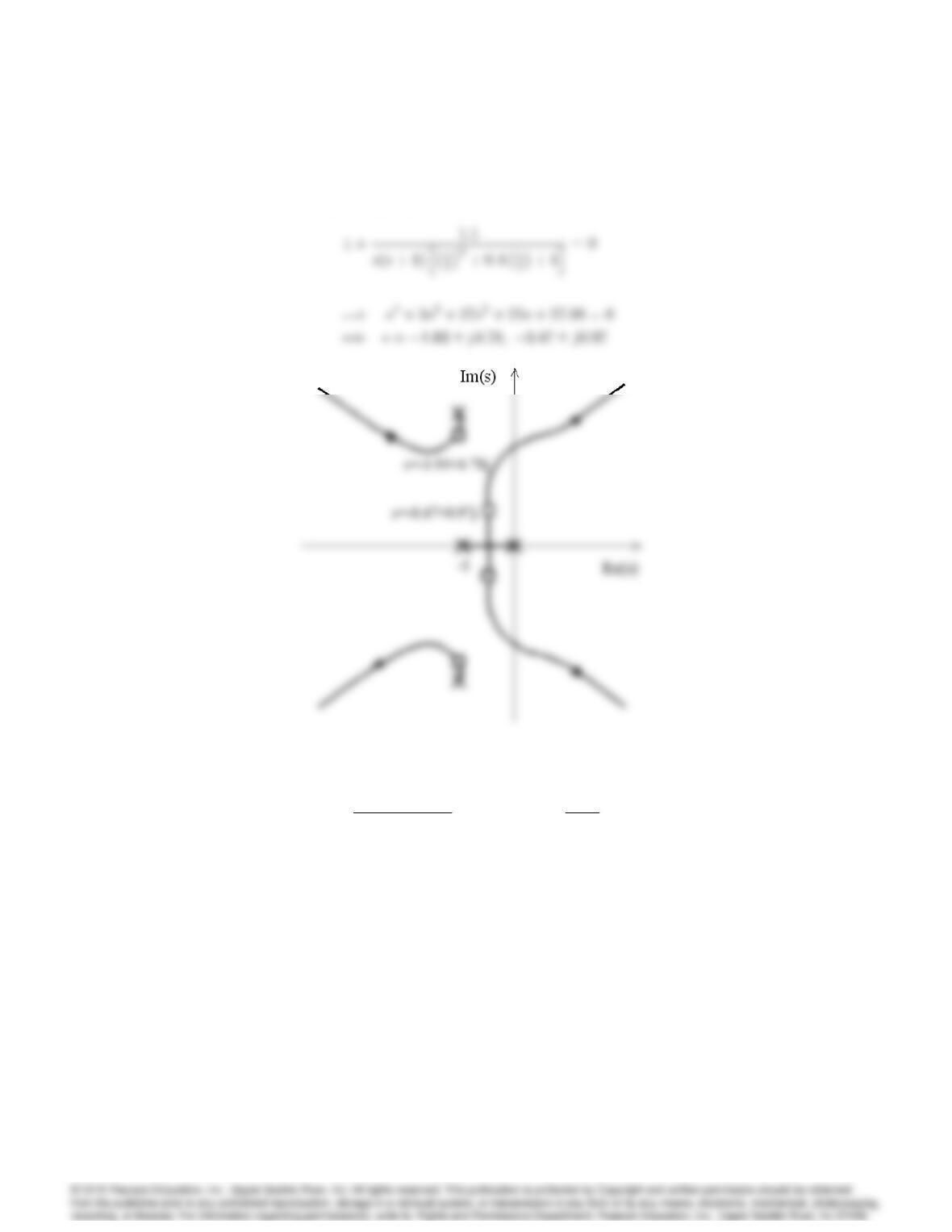
(d) Create a root locus with respect to K, and indicate the roots for a
PM of 45.
Solution :
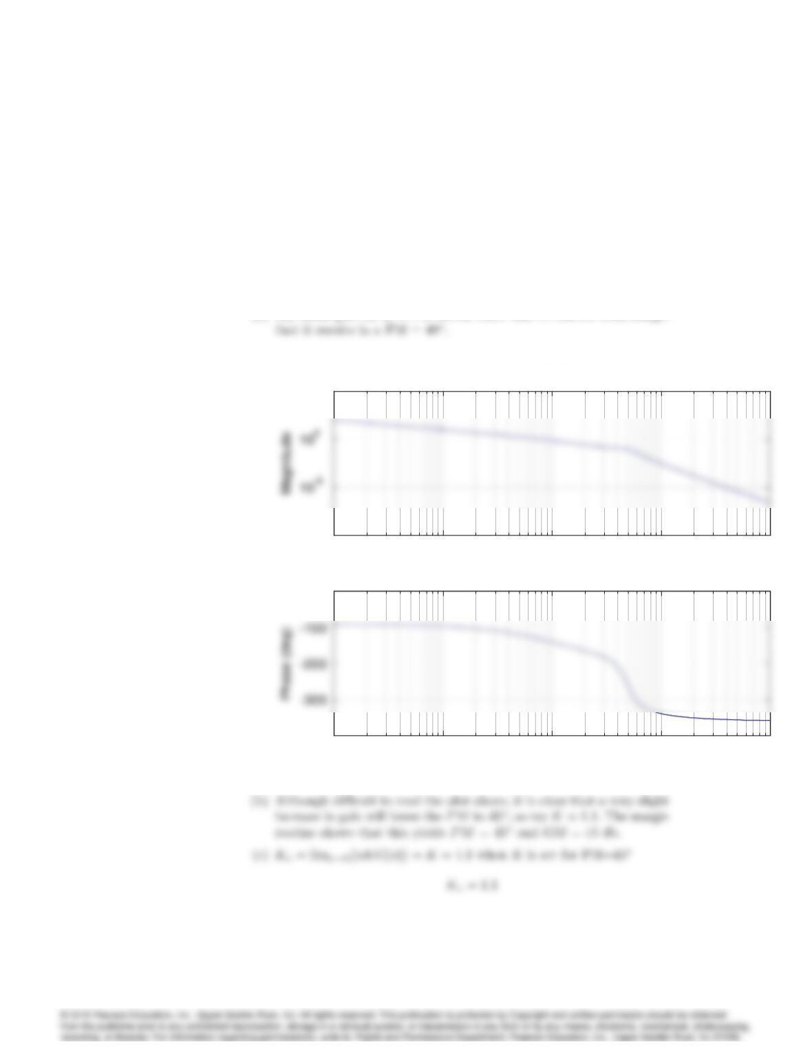
(a) The Bode plot for K= 1 is shown below and we can see from margin
10-2 10-1 100101102
10-10
105
ω (rad/sec)
Bode plot for Prob. 6.31
10-2 10-1 100101102
10-10
105
ω (rad/sec)
Bode plot for Prob. 6.31
10-2 10-1 100101102
-400
0
ω (rad/sec)
10-2 10-1 100101102
10-10
105
ω (rad/sec)
Bode plot for Prob. 6.31
10-2 10-1 100101102
10-10
105
ω (rad/sec)
Bode plot for Prob. 6.31
10-2 10-1 100101102
-400
0
ω (rad/sec)
6099
(d) The characteristic equation for PM of 45:
32. For the system depicted in Fig. 6.92(a), the transfer-function blocks are
defined by
G(s) = 1
(s+ 2)2(s+ 4) and H(s) = 1
s+ 1:
(a) Using rlocus and rlocfind, determine the value of Kat the stability
boundary.
(b) Using rlocus and rlocfind, determine the value of Kthat will produce
roots with damping corresponding to = 0:707.
(c) What is the gain margin of the system if the gain is set to the value
determined in part (b)? Answer this question without using any
frequency response methods.
(d) Create the Bode plots for the system, and determine the gain margin
that results for PM = 65. What damping ratio would you expect
for this PM?